This post separates two proof questions that are easy to confuse.
The first question is algebraic: if the transformer has already learned a fixed solver step, what error does that solver step make? This question has an exact finite-dimensional answer.
The second question is statistical and dynamical: during pretraining, how do the attention matrices learn a solver step that works across many random tasks? This is where replica theory enters. The relevant state is not one loss curve; it is a set of overlaps between the learned preconditioner, the prompt geometry, and the task distribution.
The proof structure is short once the problem is written in finite-dimensional form. The prompt gives an encoder system
\[G_m z\simeq b_m,\]and the query solve gives a decoder system
\[H(\widehat z)x=c(\widehat z).\]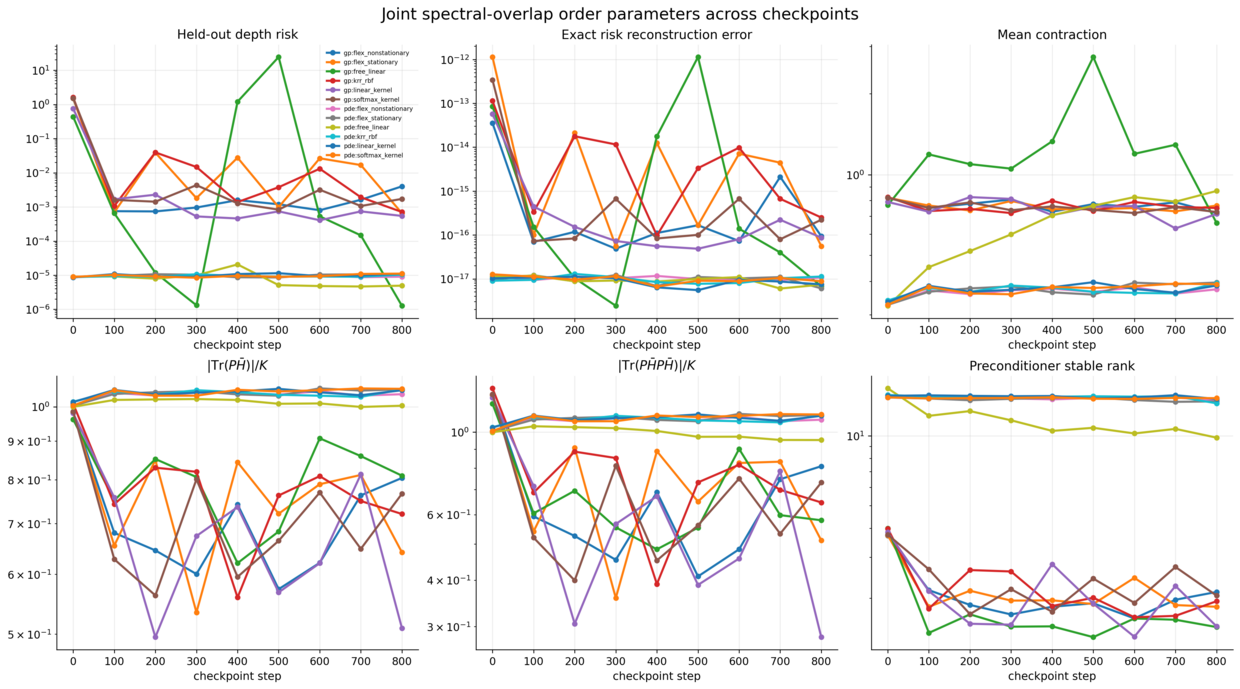
Compact diagnostic plots (simple experiments)
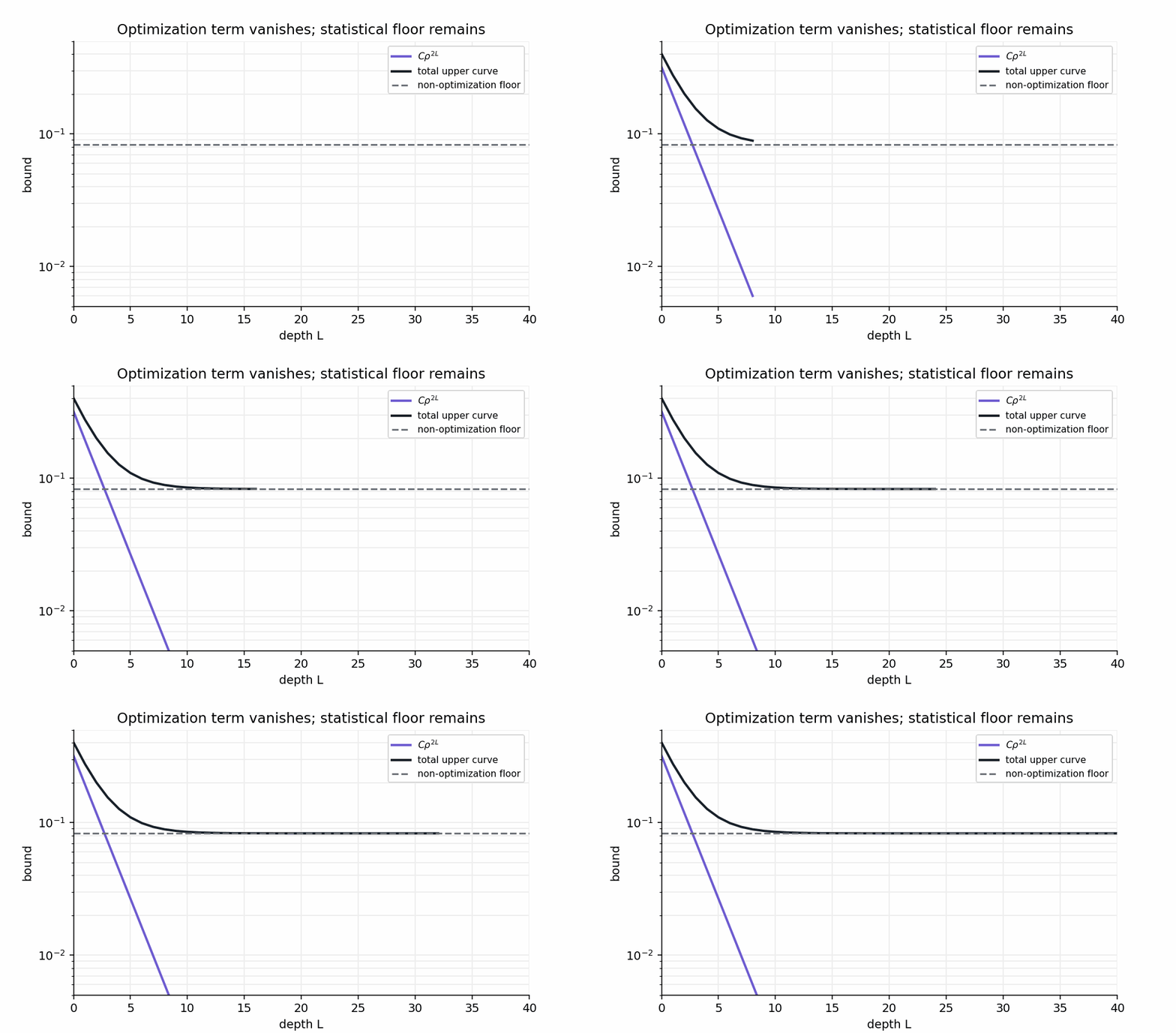 The animation shows the proof budget as depth increases. The optimization term \(\rho^{2L}\) collapses with depth, but the prompt, training-task, and Galerkin terms remain. This is why deeper decoders cannot remove encoder uncertainty or discretization error by themselves. 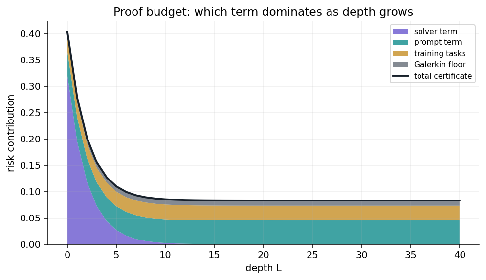 The stacked plot is the same bound without motion. It is useful because it shows when extra layers stop helping: once the solver term is below the statistical floor, the proof says to improve prompts, tasks, or discretization, not just depth. 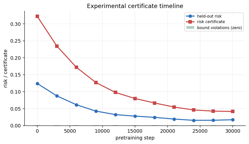 The certificate timeline separates measured held-out risk from the finite-sample upper curve. The upper curve is conservative by design. Its role is not to be tight, but to certify that the clipped held-out loss is controlled. 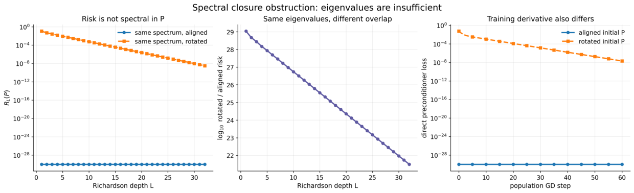 This is the crux of why the replica state cannot be only a spectrum. Two preconditioners can share eigenvalues and singular values while giving different risks because their eigenvectors overlap differently with the PDE system. 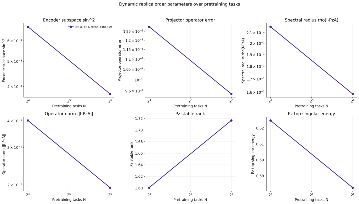 The dynamic order-parameter plot shows the quantities the theory has to close: not just marginal spectra, but mixed traces involving the learned preconditioner, the Hessian, and the residual covariance.The encoder estimate is
\[\widehat z=(G_m^\top G_m+\lambda I)^{-1}G_m^\top b_m.\]For a well-conditioned prompt design, the coefficient error has the usual least-squares form:
\[\widehat z-z = -(G_m^\top G_m+\lambda I)^{-1}\lambda z + (G_m^\top G_m+\lambda I)^{-1}G_m^\top\varepsilon .\]The first term is bias from ridge regularization. The second is variance from prompt noise. This is the encoder part.
The decoder part is exact. If (x_\star=H^{-1}c) and
\[x_{\ell+1}=x_\ell+P_\theta(c-Hx_\ell),\]then
\[x_L-x_\star=(I-P_\theta H)^L(x_0-x_\star).\]This gives the optimization certificate
\[\|x_L-x_\star\|_2 \le \|I-P_\theta H\|_2^L\|x_0-x_\star\|_2.\]Putting encoder and decoder together,
\[\|\widehat x_L-x_\star\|_2^2 \le 2\|\widehat x_L-x^\dagger(\widehat z)\|_2^2 + 2\|x^\dagger(\widehat z)-x_\star\|_2^2.\]The first term is a solver error. The second term is a task-identification error.
For held-out generalization, the experiments use a clipped empirical Bernstein certificate. If
\[\ell_c=\min(\ell,c),\]then with probability at least (1-\delta),
\[R_c \le \widehat R_c + \sqrt{\frac{2\widehat V_c\log(2/\delta)}{n}} + \frac{7c\log(2/\delta)}{3(n-1)}.\]The reason for clipping is simple: raw Gaussian losses are unbounded, so a distribution-free finite-sample certificate needs either clipping or a separate tail assumption.
The final bound has the shape
\[\mathbb E\|\widehat u_\star-u_\star\|^2 \lesssim \varepsilon_{\mathrm{Gal}}(d) + \frac{K_{\mathrm{eff}}}{m} + \rho^{2L} + \frac{\mathrm{Comp}(\Theta)}{\sqrt N} + \varepsilon_{\mathrm{arch}}.\]Each term has a role: discretization, prompt estimation, solver depth, pretraining sample size, and architecture approximation.
Why the exponent is (2L)
The decoder error norm contracts like
\[\|e_L\|\leq \rho^L\|e_0\|.\]But the risk is a squared error. Therefore the solver contribution scales like
\[\|e_L\|^2\leq \rho^{2L}\|e_0\|^2.\]This is the source of the (2L) exponent in the risk bound. It is not an extra assumption; it is just the passage from norm error to squared loss.
Where the transformer enters the proof
The proof does not require pretending that attention is magic. It only requires showing that the architecture approximates the update
\[z^{\ell+1}=z^\ell+B_\Theta(c_m-H_m z^\ell).\]The query/key part can be interpreted as selecting weak equations or spectral directions. The value stream carries the residual evidence. The feed-forward part turns this evidence into a correction. If the architecture exactly implements the update, the only remaining solver error is the Richardson term. If it implements it approximately, an additional architecture error appears:
\[\varepsilon_{\mathrm{arch}}.\]This term is where finite width, low-rank heads, softmax normalization, and feature restrictions live.
What the experiments certify
The experiments check the proof in pieces. Encoder-only recovery verifies the closed population trajectory
\[G_s-G_\star=(G_0-G_\star)(I-\eta\Sigma_z)^s.\]Decoder-only pretraining verifies the frozen Richardson identity and its pointwise bound. Encoder–decoder experiments verify that the end-to-end risk splits into encoder floor plus decoder component. PDE recasts verify that the weak-form encoder really gives the expected finite-dimensional (G_mz=b_m) system.
The strongest current statement is therefore modular. We have exact algebraic certificates for the encoder and decoder pieces in the finite-dimensional framework. What remains harder is a single scalar closed-form theory for global nonlinear learnable-kernel attention population training. That is a different problem from the finite-set adjoint identity, which is exact but high-dimensional.
Where the replica trick enters
The replica trick is not needed to prove the frozen Richardson identity. It is needed to predict the typical training and generalization curve when ((G_m,H_m,z)) are random and the learned attention parameters are optimized over many tasks.
For a decoder preconditioner (P_\theta), the task risk has the schematic form
\[R_L(\theta) = \frac1K \mathbb E_{H,S} \operatorname{Tr}\{(I-P_\theta H)^L S (I-P_\theta H)^{L\top}\}.\]The hard object is the quenched free energy
\[\Phi_\beta = -\frac1{\beta K} \mathbb E_{\mathcal D} \log \int \exp\{-\beta K R_{\mathcal D}(\theta)\}\,d\pi(\theta).\]The replica step rewrites
\[\mathbb E\log Z = \lim_{r\to 0} \frac{\mathbb E Z^r-1}{r}, \qquad Z= \int e^{-\beta K R_{\mathcal D}(\theta)}d\pi(\theta),\]and introduces (r) copies (P_{\theta^1},\ldots,P_{\theta^r}). The saddle point is not a scalar spectrum. It must track mixed overlaps such as
\[m_a=\frac1K\operatorname{Tr}(P_{\theta^a}H), \qquad q_{ab}=\frac1K\operatorname{Tr}(P_{\theta^a}H P_{\theta^b}H),\]and, once the task covariance matters,
\[s_{ab} = \frac1K \operatorname{Tr}(P_{\theta^a}H S H^\top P_{\theta^b\top}).\]For the encoder, analogous overlaps involve the prompt Gram matrix:
\[Q_{ab}^{\rm enc} = \frac1K \operatorname{Tr}\{(\widehat G^{a}-G_\star)\Sigma_z (\widehat G^{b}-G_\star)^\top\}.\]This is the actual crux. In Gaussian low-rank models, (G_m^\top G_m) has a Marchenko–Pastur limit and the encoder overlaps can close. For nonlinear attention, the replicated action must also describe how (Q,K,V) align with the eigenvectors of (H), with the value residual covariance, and with the task covariance (S). The useful theorem would be a closed dynamical system for these order parameters during training. The modular bounds above are exact, but they do not by themselves solve that replica closure.
Why spectra alone are not enough
A natural first guess is that the decoder risk should be predictable from the spectrum of (P_\theta). That is false in general. The frozen decoder risk is
\[R_L(P) = K^{-1} \operatorname{Tr}\{(I-PH)^L S (I-PH)^{L\top}\}.\]This depends on the alignment between (P), (H), and the task covariance (S), not just on the marginal eigenvalues of (P). Two matrices can share the same singular values and eigenvalues while having different overlaps with the system matrix, and therefore different risk.
The correct population state must therefore include mixed quantities such as
\[\operatorname{Tr}(PH),\qquad \operatorname{Tr}(PHPH),\qquad \operatorname{Tr}(PHS H^\top P^\top).\]This is the proof-level reason the global nonlinear learnable-kernel theory is harder than the frozen decoder certificate. The frozen certificate is exact for every checkpoint. The scalar training closure needs richer order parameters.
Practical proof status
The result we can safely use in a paper-style argument is the modular one: encoder least-squares recovery plus decoder Richardson contraction plus a generalization certificate. The result we should not overclaim is a closed one-dimensional law for all nonlinear attention parameters during population training. The experiments support local NTK predictions and exact finite-set gradients, but the full global closure is a separate problem.
External Papers Used
This series uses paper names only after introducing the problem they solve. The main external anchors are the following.
Low-rank in-context learning and replica theory. Kaito Takanami, Takashi Takahashi, and Yoshiyuki Kabashima, “Learning Linear Regression with Low-Rank Tasks In-Context,” arXiv:2510.04548. This is the reference for the high-dimensional low-rank task model and its replica generalization calculation.
Training dynamics of linear attention. Yedi Zhang, Aaditya K. Singh, Peter E. Latham, and Andrew Saxe, “Training Dynamics of In-Context Learning in Linear Attention,” arXiv:2501.16265. This is the reference point for exact gradient-flow phenomena in linear-attention ICL.
Learnable linear-attention kernels. Haoran Zhang and Feng Zhou, “Flexformer: Flexible Linear Transformer with Learnable Attention Kernel,” arXiv:2606.27748. This motivates the learned-kernel decoder experiments, but the posts distinguish local diagnostics from a proved global training theory.
Differentiable Galerkin assembly. Shizheng Wen, Mingyuan Chi, Tianwei Yu, Ben Moseley, Mike Yan Michelis, Pu Ren, Hao Sun, and Siddhartha Mishra, “Learning, Solving and Optimizing PDEs with TensorGalerkin,” arXiv:2602.05052. This is the relevant numerical-analysis reference for differentiable Galerkin assembly and PDE-constrained learning.