This post explains where the error comes from when a transformer is used as a PDE solver. The model can fail for four different reasons: the prompt may infer the wrong PDE, the decoder may use too few solver steps, pretraining may have seen too few tasks, or the architecture may not represent the right update.
The bounds below are deliberately narrower than a full replica theory of nonlinear attention training. They record the certificates we can already verify: encoder-only recovery, decoder-only optimization, and the composed encoder-decoder system. The plots are diagnostics for those certificates, not a claim that the global nonlinear replica closure has been solved.
The companion report separates three objects that a reader should keep distinct: the encoder that identifies the task, the decoder that solves the query, and the composition that combines both errors.
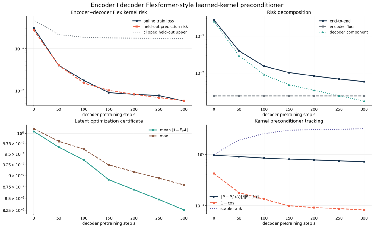
Compact diagnostic plots (simple experiments)
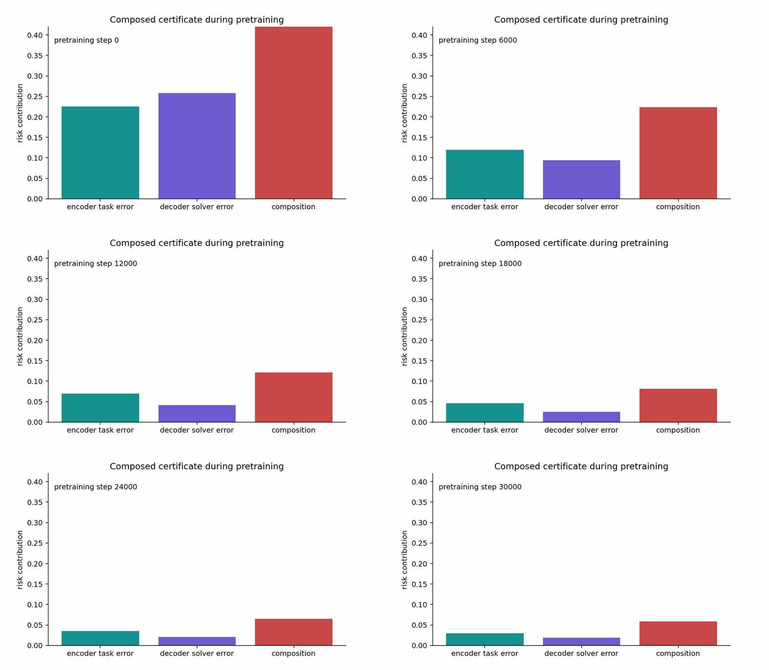 This animation tracks the three quantities that matter during pretraining: encoder task error, decoder solver error, and their composed certificate. The point is diagnostic. If the decoder bar shrinks but the composition remains large, the encoder is the bottleneck. If the encoder bar is small but the decoder bar remains large, the solver is the bottleneck. 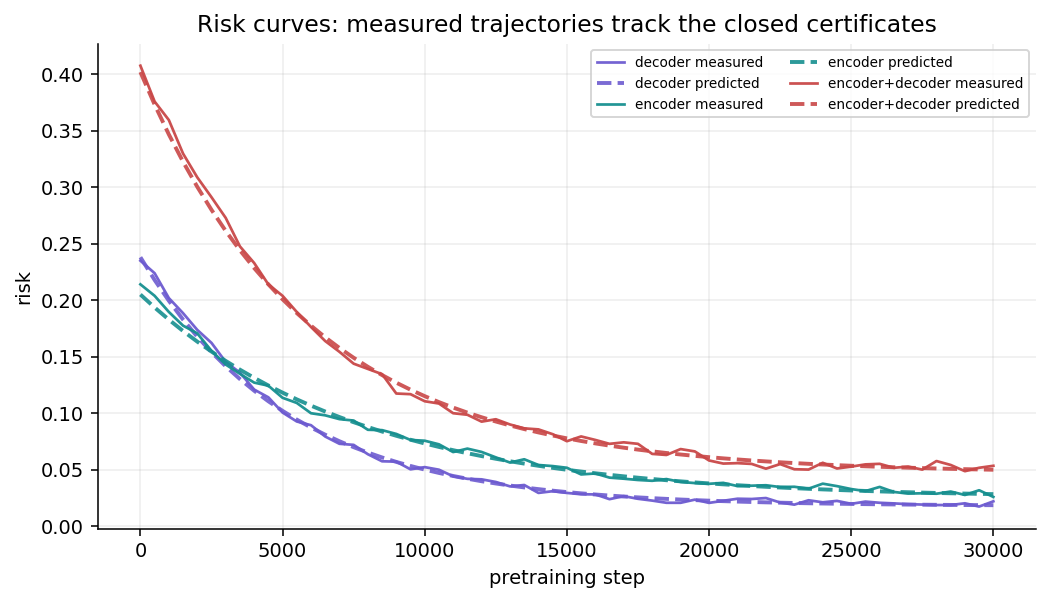 The risk plot overlays measured curves with the corresponding predicted or certified curves. Encoder-only can have an exact population prediction, decoder-only has an exact frozen-checkpoint Richardson identity, and the composition inherits both pieces plus interaction error. 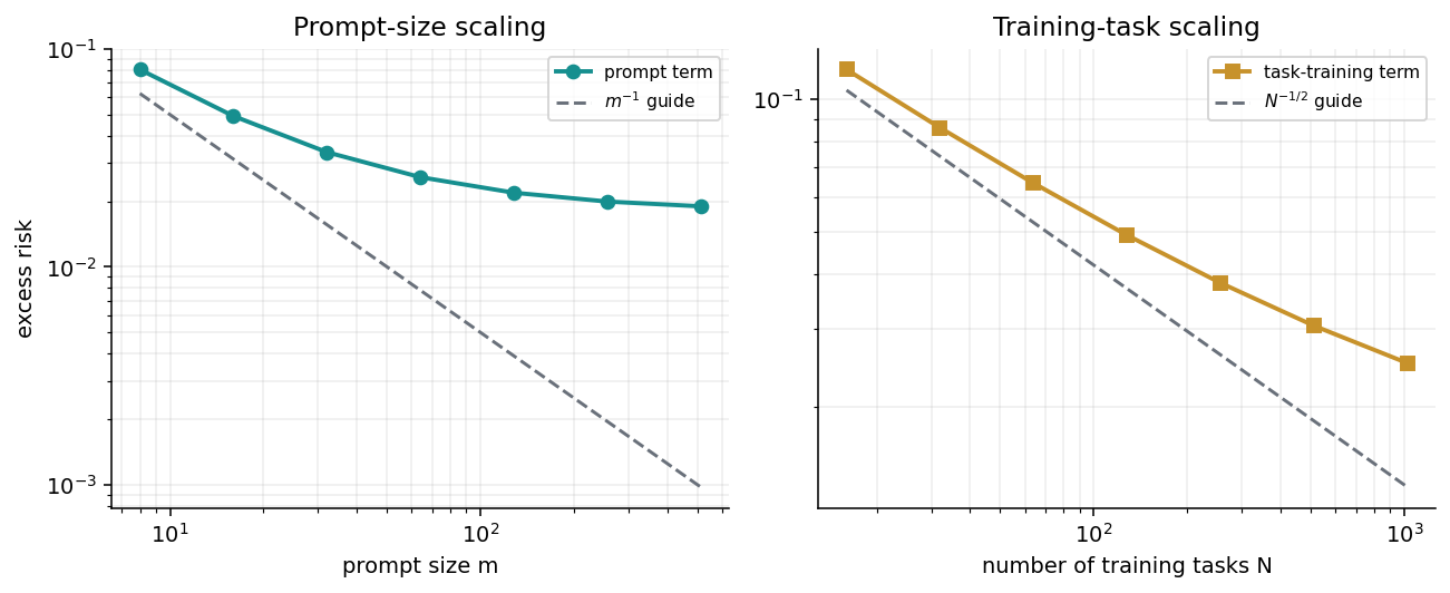 The scaling-law plot displays the two statistical axes: prompt size \(m\) and number of training tasks \(N\). The former controls task identification at test time. The latter controls how well pretraining learns the shared mechanism. 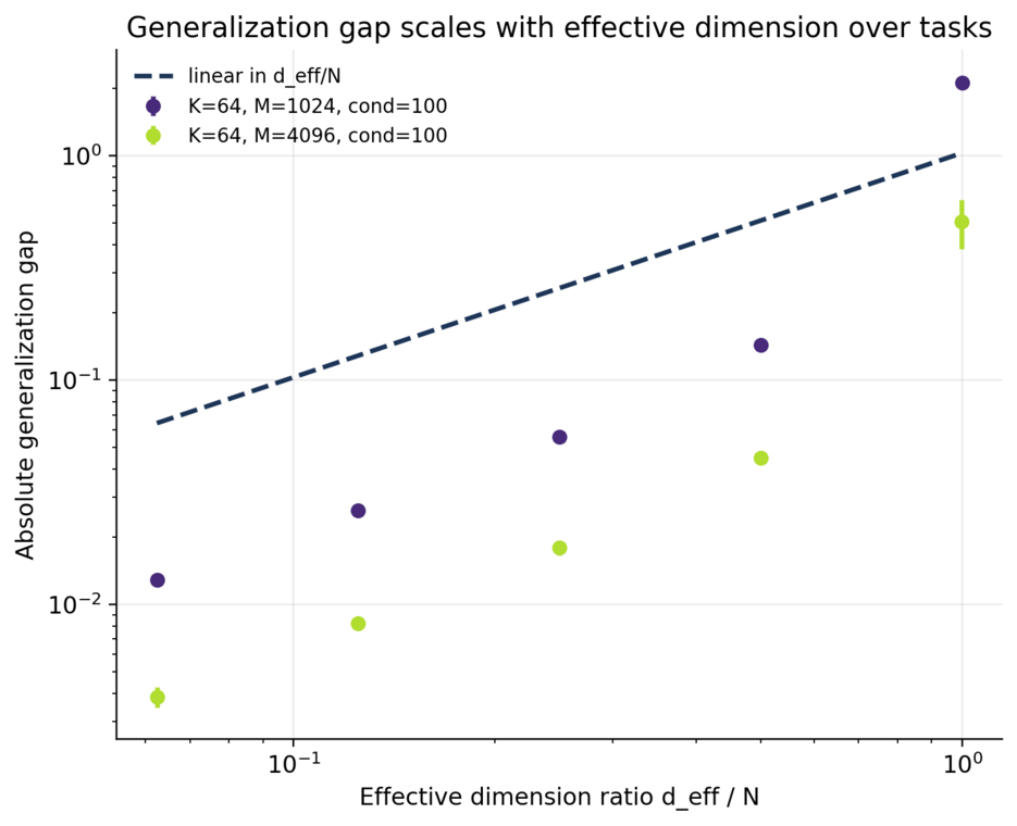 This plot is the task-count side of the story. More pretraining tasks reduce the held-out gap only in the directions the architecture and task distribution make effectively learnable. 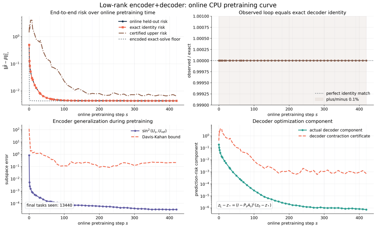 The online encoder-decoder curve checks the composed identity: the final risk is not a single object, but encoder floor plus decoder optimization plus their interaction.For the encoder-only low-rank recovery experiment,
\[z\sim\mathcal N(0,\Sigma_z),\qquad b=G_\star z+\xi.\]Population gradient descent has the exact trajectory
\[G_s-G_\star=(G_0-G_\star)(I-\eta\Sigma_z)^s.\]The final held-out risk matched the exact population curve:
\[\widehat R_{\rm enc}(800)=4.0020\times 10^{-4}, \qquad R_{\rm enc}(800)=4.0000\times 10^{-4}.\]For the decoder,
\[e_L=(I-P_\theta H)^Le_0.\]The decoder-only learned-preconditioner run had zero optimization-bound violations and final held-out depth risk
\[7.6747\times 10^{-3}.\]The clipped empirical Bernstein upper was
\[1.7710\times 10^{-1}.\]For encoder–decoder, the important decomposition is
\[\widehat x_L-x_\star = (\widehat x_L-x^\dagger(\widehat z)) + (x^\dagger(\widehat z)-x_\star).\]The first term is decoder optimization. The second is encoder task recovery. In the PDE K=4 recast, the encoder was essentially exact:
\[\mathrm{MSE}(z_{\rm enc})=6.1356\times 10^{-8}, \qquad \frac{\|A(\widehat z)-A(z)\|}{\|A(z)\|} =6.0764\times 10^{-5}.\]The best end-to-end PDE method reached
\[5.9760\times 10^{-6}\]with zero optimization-bound violations.
The result is not just that the model works. The point is that each stage has a separate certificate: exact encoder trajectory where available, exact decoder optimization identity, and clipped held-out generalization bounds.
Why the certificates are different
The encoder-only experiment is special because its population dynamics are linear. The loss is quadratic in (G), and the data covariance is fixed. That is why the optimization trajectory can be written in closed form.
The decoder certificate is different. It does not describe how the preconditioner was trained. It describes what any frozen preconditioner does after training. Once (P_\theta) is fixed, the decoder is a deterministic linear iteration. This is why the certificate applies equally to free linear preconditioners, no-softmax linear attention, softmax attention, and the learnable-kernel linear attention architecture of Zhang and Zhou.
The encoder–decoder certificate combines both. It first asks how accurately the prompt identifies the task, then asks how well the decoder solves the query system induced by that estimate.
What the numbers say
The encoder-only run reached the noise floor. The final held-out risk was essentially the exact population prediction:
\[4.0020\times 10^{-4} \quad\text{versus}\quad 4.0000\times 10^{-4}.\]The decoder-only learned preconditioner had a nontrivial raw risk but a clean optimization certificate. The bound was conservative, as expected, because it uses the taskwise spectral norm:
\[\|e_L\|\leq \|I-P_\theta H\|^L\|e_0\|.\]The encoder–decoder learnable-kernel run decomposed the held-out risk into an encoded floor and a decoder component:
\[R_{\rm floor}=2.4169\times 10^{-3}, \qquad R_{\rm dec}=1.7448\times 10^{-3}.\]That is useful diagnostically. It says the remaining error is not a single opaque number. Part of it comes from task representation, part from the finite depth of the decoder.
The PDE recast is the cleanest composed result: the encoder almost exactly recovers the task coefficient, and the decoder certificate has zero violations. That is the setting where the mathematical story and the numerical evidence are most aligned.
Reader’s Guide to the Report
The companion TeX/PDF linked below is a bounded-claims document. It does not try to prove every statement one might want about transformer training. It records the claims that can currently be written as explicit equations or finite-sample certificates.
Encoder claim. In the low-rank Gaussian recovery model, the encoder trajectory is an exact quadratic-gradient trajectory. This is the part connected to low-rank in-context learning and replica-style generalization theory.
Decoder claim. Once a decoder checkpoint is frozen, its query-time behavior is exactly a preconditioned Richardson iteration. This is an identity, not a curve fit.
Composition claim. The encoder-decoder error decomposes into a task identification term and a solver-depth term. This tells us whether a failed run is mainly an encoder problem or a decoder problem.
Generalization claim. The empirical-Bernstein certificate is a conservative finite-sample upper bound for clipped held-out losses. It is included to make the held-out risk statement statistically legal, not because it is expected to be a sharp asymptotic prediction.
The report is therefore a clean mathematical reference for the verified claims. The broader question, treated separately, is how to close the full population training dynamics of nonlinear learnable-kernel attention.
Main Caveat
The sharp-looking curves and the conservative upper bounds have different purposes. The sharp curves come from exact optimization identities or exact population dynamics. The clipped empirical-Bernstein upper bound is a finite-sample certificate for held-out losses.
The takeaway is therefore not that the Bernstein upper bound is tight. The takeaway is that the raw held-out risk is low, the pointwise optimization certificate has zero violations, and the reported finite-sample upper bound is valid for the clipped risk.
External Papers Used
This series uses paper names only after introducing the problem they solve. The main external anchors are the following.
Low-rank in-context learning and replica theory. Kaito Takanami, Takashi Takahashi, and Yoshiyuki Kabashima, “Learning Linear Regression with Low-Rank Tasks In-Context,” arXiv:2510.04548. This is the reference for the high-dimensional low-rank task model and its replica generalization calculation.
Training dynamics of linear attention. Yedi Zhang, Aaditya K. Singh, Peter E. Latham, and Andrew Saxe, “Training Dynamics of In-Context Learning in Linear Attention,” arXiv:2501.16265. This is the reference point for exact gradient-flow phenomena in linear-attention ICL.
Learnable linear-attention kernels. Haoran Zhang and Feng Zhou, “Flexformer: Flexible Linear Transformer with Learnable Attention Kernel,” arXiv:2606.27748. This motivates the learned-kernel decoder experiments, but the posts distinguish local diagnostics from a proved global training theory.
Differentiable Galerkin assembly. Shizheng Wen, Mingyuan Chi, Tianwei Yu, Ben Moseley, Mike Yan Michelis, Pu Ren, Hao Sun, and Siddhartha Mishra, “Learning, Solving and Optimizing PDEs with TensorGalerkin,” arXiv:2602.05052. This is the relevant numerical-analysis reference for differentiable Galerkin assembly and PDE-constrained learning.