Part 1 fixed the PDE operator and tested only the decoder. This post adds the inverse problem: the PDE operator can change from task to task, and the prompt examples are evidence about which equation generated them.
The transformer now has two jobs. The encoder must infer the hidden coefficient vector from the prompt. The decoder must solve a new query using the inferred operator. The figures are small diagnostics for that two-stage computation, not a replacement for the full benchmark tables.
The variable-coefficient case is where in-context learning becomes genuinely task-adaptive. Now the operator is not fixed:
\[A(z)=A_0+\sum_{k=1}^K z_k A_k .\]The prompt consists of source-solution pairs ((f_i,u_i)) produced by the same unknown task coefficient (z). Each pair satisfies
\[A(z)u_i=f_i.\]Rearranging this equation gives a linear inverse problem for (z). In weak form, with test functions (v_r),
\[G_{(i,r),k}=\langle A_k u_i,v_r\rangle,\]and
\[b_{(i,r)}=\langle f_i-A_0u_i,v_r\rangle.\]Stacking over prompt examples (i) and tests (r) gives
\[G_m z\simeq b_m.\]The encoder is therefore a ridge least-squares estimator:
\[\widehat z=(G_m^\top G_m+\lambda I)^{-1}G_m^\top b_m.\]Once the task is encoded, the query solve becomes ordinary again:
\[u_{\ell+1}=u_\ell+P_\theta(f_\star-A(\widehat z)u_\ell).\]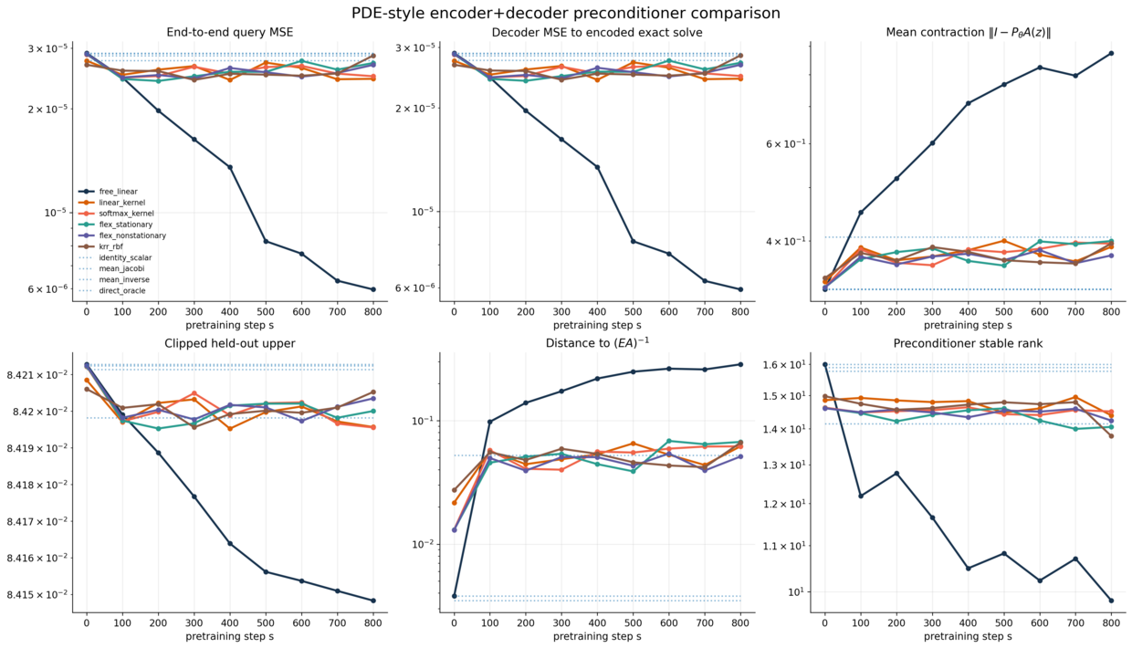
Compact diagnostic plots (simple experiments)
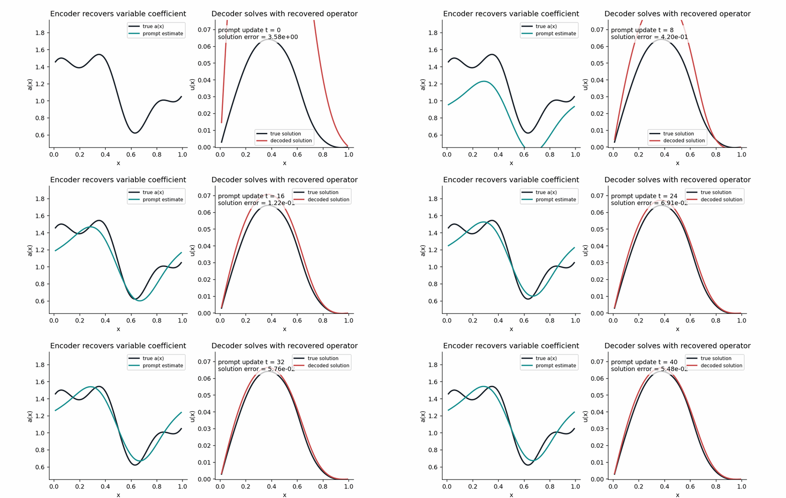 The left panel animates the encoder estimate of \(a(x)\). The right panel shows the query solution obtained after solving with the recovered operator. This is the whole variable-\(a\) story: prompt examples first reconstruct the operator, then the decoder solves the new right-hand side. 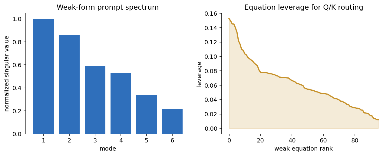 The weak-form prompt is not just a bag of examples. It has a spectrum and a leverage profile. High-leverage equations are the rows that most strongly probe latent coefficient directions, which is exactly the information query/key routing should learn to select. 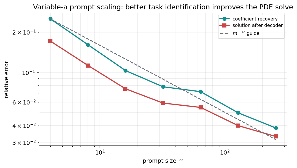 As prompt size grows, the coefficient estimate improves and the decoded PDE solution follows. This separates the encoder bottleneck from the decoder bottleneck: if the coefficient curve is still wrong, the PDE solve can be perfect and still solve the wrong equation. 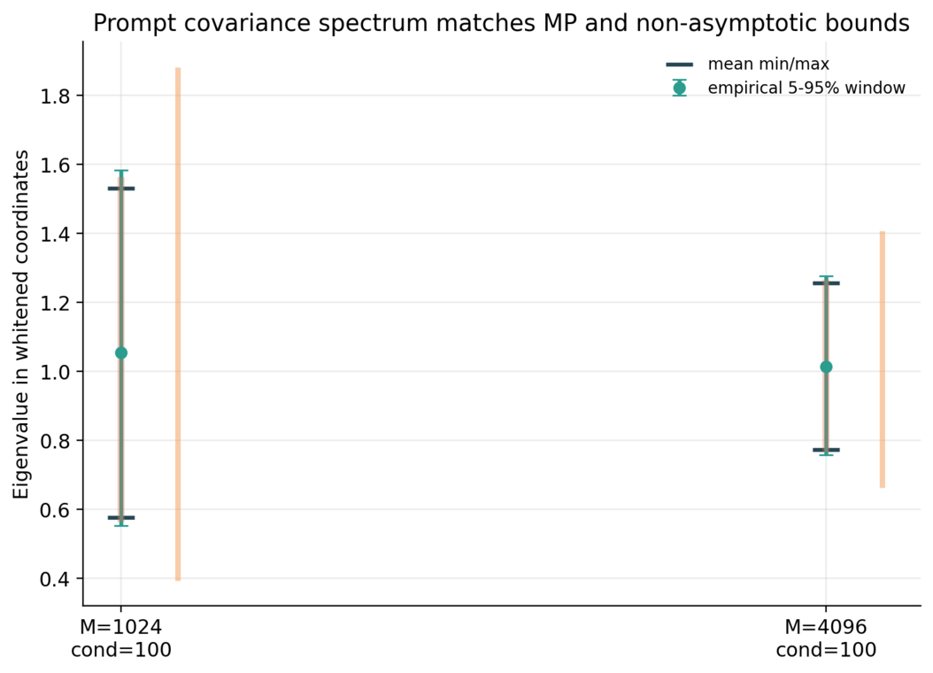 The prompt spectrum is the first sanity check for coefficient recovery. If the smallest visible prompt eigenvalues collapse, some directions of \(z\) cannot be identified no matter how strong the decoder is. 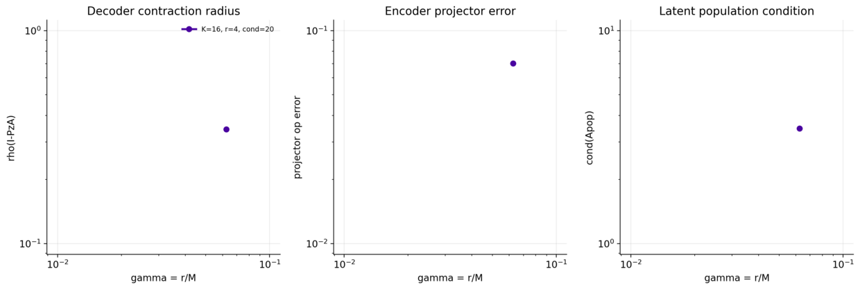 This scaling view tracks the ratio between latent task dimension and prompt equations. It is the finite-dimensional version of the Marchenko--Pastur prompt-size law.This decomposition is important. It separates the problem into two errors:
\[\widehat u_L-u_\star = \underbrace{\widehat u_L-u^\dagger(\widehat z)}_{\text{decoder error}} + \underbrace{u^\dagger(\widehat z)-u_\star}_{\text{encoder error}}.\]The decoder error is controlled by Richardson contraction. The encoder error is controlled by how well the prompt identifies the coefficient (z). In the finite-rank setting, the effective dimension is (K), so the natural scaling is that longer prompts reduce the coefficient-estimation error.
This is the key difference from the constant-coefficient setting: the decoder still solves, but the encoder first reconstructs the task.
Why weak form matters
The weak-form construction avoids differentiating the observed solution numerically in a fragile way. The PDE identity is tested against (v_r), and the unknown coefficient only appears through the entries
\[\langle A_k u_i,v_r\rangle.\]This is exactly what makes the encoder linear in the unknown coefficient vector. The row index ((i,r)) simply means: prompt example (i), test function (r). There is no tensor mystery. We flatten those pairs into rows of the matrix (G_m).
The prompt size matters because it controls how many independent weak equations we get. If (m) is too small, (G_m^\top G_m) is poorly conditioned and some coefficient directions are invisible. If (m) is large and the source distribution excites the relevant modes, the ridge estimator becomes stable.
The encoder–decoder error budget
The practical bound has two main terms. The first is coefficient recovery:
\[\|\widehat z-z\|^2.\]For a ridge estimator, this decomposes into bias and variance:
\[\widehat z-z = -(G_m^\top G_m+\lambda I)^{-1}\lambda z + (G_m^\top G_m+\lambda I)^{-1}G_m^\top\varepsilon.\]The second is solver error after the encoded operator has been formed:
\[\|(I-P_\theta A(\widehat z))^L e_0\|^2.\]This is the right way to understand task diversity. If the distribution of (z) lives in a small effective dimension, fewer prompt equations are needed. If (z) spans many directions or if the weak equations have poor leverage, the encoder needs longer prompts.
Task difficulty is therefore not just the condition number of a PDE matrix. It is also the condition number of the prompt inverse problem (G_m^\top G_m). A task can be easy to solve once (A(z)) is known, but hard to identify from the prompt. Conversely, it can be easy to identify (z) but hard to solve the query system if (A(z)) is ill-conditioned. The encoder–decoder view keeps these two difficulties separate.
Prompt scaling
The prompt length (m) controls how many equations the encoder gets. If each prompt pair is tested against (R) weak functions, the encoder sees roughly (mR) rows. The latent dimension is (K). The favorable regime is therefore not just (mR\ge K), but (G_m^\top G_m) being well-conditioned on the active coefficient directions.
In finite-rank Gaussian models, this is the same idea as effective dimension. Some directions of (z) have large variance and are common across tasks. Others are rare or weakly observed. The encoder learns the directions that the prompt distribution makes identifiable. That gives a concrete meaning to task diversity: diversity is not merely having many tasks, but exciting the latent directions that matter for future query solves.
Decoder stability after encoding
The decoder sees (A(\widehat z)), not (A(z)). This means an encoder error can change the contraction of the solver. If (P_\theta) is trained for the true operator family but the encoder produces a biased (\widehat z), the decoder may still contract, but around the wrong system.
This is why the experimental reports include an encoded floor: the risk obtained by solving exactly with the encoded operator. The floor separates representation error from solver error. If the floor is large, the encoder is the bottleneck. If the floor is small but the final risk is large, the decoder or preconditioner is the bottleneck.
In the (K=4) PDE recast experiment, the encoded floor was tiny. That means the mathematical recast worked: weak-form prompt equations really did recover the task. The remaining comparison is mainly about which decoder preconditioner solves the induced query system fastest.
Takeaway
Variable coefficients turn in-context learning into a two-stage computation: first infer the PDE coefficient from the prompt, then solve the query equation. The mathematics is still least squares plus Richardson, but prompt conditioning is now essential.
External Papers Used
This series uses paper names only after introducing the problem they solve. The main external anchors are the following.
Low-rank in-context learning and replica theory. Kaito Takanami, Takashi Takahashi, and Yoshiyuki Kabashima, “Learning Linear Regression with Low-Rank Tasks In-Context,” arXiv:2510.04548. This is the reference for the high-dimensional low-rank task model and its replica generalization calculation.
Training dynamics of linear attention. Yedi Zhang, Aaditya K. Singh, Peter E. Latham, and Andrew Saxe, “Training Dynamics of In-Context Learning in Linear Attention,” arXiv:2501.16265. This is the reference point for exact gradient-flow phenomena in linear-attention ICL.
Learnable linear-attention kernels. Haoran Zhang and Feng Zhou, “Flexformer: Flexible Linear Transformer with Learnable Attention Kernel,” arXiv:2606.27748. This motivates the learned-kernel decoder experiments, but the posts distinguish local diagnostics from a proved global training theory.
Differentiable Galerkin assembly. Shizheng Wen, Mingyuan Chi, Tianwei Yu, Ben Moseley, Mike Yan Michelis, Pu Ren, Hao Sun, and Siddhartha Mishra, “Learning, Solving and Optimizing PDEs with TensorGalerkin,” arXiv:2602.05052. This is the relevant numerical-analysis reference for differentiable Galerkin assembly and PDE-constrained learning.