Three-Layer Learning as a DMFT–RMT–BBP Closure Problem

The final master paper now contains the complete proof-level package: exact finite Hermite geometry, a controlled extension to general links, the fresh block-Wishart reduction, the MSRJD/cavity/replica/spectral-AMP program, the Kac–Rice interface, and a time-resolved experiment that puts coefficient recovery, Schur geometry, and fresh Hessian spectroscopy on the same clock.

The result is a reduction, not a claim that every three-layer network has already been solved. The finite algebra is exact. The high-dimensional DMFT–RMT–BBP closure is stated under four explicit hypotheses that remain to be proved for joint reused-data Muon.

The model used as the exact testbed

For Gaussian teacher coordinates $z\in\mathbb R^k$,

\[\begin{aligned} h &=Vz+b, & q&=h^{\odot2}-1,\\ r &=Uz+Aq+c, & s&=r^{\odot2}-1,\\ f_\theta(z)&=a_0+\alpha^\top q+\beta^\top s. \end{aligned}\]

This network is degree four in $z$. Its population loss therefore has a finite multivariate Hermite representation

\[\mathcal R(\theta) =\frac12\sum_{|\gamma|\leq4}\gamma!\, \big(c_\gamma(\theta)-c_{\star,\gamma}\big)^2.\]

The coefficient Jacobian gives the complete gradient and the Hessian split

\[\nabla^2\mathcal R =J^\top D J+ \sum_\gamma\gamma!\, \big(c_\gamma-c_{\star,\gamma}\big)\nabla^2c_\gamma.\]

The first term is Gauss–Newton curvature. The second is residual curvature, which can be indefinite away from interpolation.

For degrees $r=2,3,4$, residualizing the weighted coefficient Jacobian against all earlier sectors produces

\[S_r=\overline M_r^\top\overline M_r\succeq0.\]

If $\rho_r$ is the operator norm of residual curvature on the corresponding active tangent space, then

\[\lambda_{\min}\!\left(Q_r^\top\nabla^2\mathcal R\,Q_r\right) \geq \lambda_{\min}^+(S_r)-\rho_r.\]

This is a sufficient local certificate. It is not a necessary condition for a sector error to decrease.

What extends beyond quadratic activations

Let $c(\theta)$ be the full Hermite coefficient map of a general link, viewed as an element of $L^2(\gamma_k)$, and let $P_R$ retain degrees at most $R$. Define

\[\begin{aligned} \varepsilon_0&=\|(I-P_R)(c-c_\star)\|,\\ \varepsilon_1&=\|(I-P_R)Dc\|_{\rm op},\\ \varepsilon_2&=\sup_{\|u\|=\|v\|=1} \|(I-P_R)D^2c[u,v]\|. \end{aligned}\]

The new Hermite-tail theorem proves

\[\begin{aligned} \mathcal R-\mathcal R_R&=\frac12\varepsilon_0^2,\\ \|\nabla\mathcal R-\nabla\mathcal R_R\| &\leq\varepsilon_0\varepsilon_1,\\ \|\nabla^2\mathcal R-\nabla^2\mathcal R_R\|_{\rm op} &\leq\varepsilon_1^2+\varepsilon_0\varepsilon_2. \end{aligned}\]

Thus the finite Hermite theory transfers to smooth non-polynomial links when the coefficient map and its first two derivatives have controlled tails. For the quadratic network all three tails vanish at $R=4$.

This does not automatically transfer the empirical random-matrix theorem. Per-example derivative blocks can remain unbounded even when population $L^2$ tails are small.

The physical closure

The intended high-dimensional connection is

\[\boxed{\text{DMFT state }(Q,M,R,\varphi)} \longrightarrow \boxed{\text{block law }\nu_t} \longrightarrow \boxed{\text{RMT bulk edges}} \xrightarrow{\text{finite Schur equation}} \boxed{\text{BBP branch}}.\]

Each arrow has a different status.

1. A reused-data DMFT must close two-time correlations, responses, overlaps, and the finite parameters $(A,b,c,\alpha,\beta,a_0)$. This is open.
2. At a fixed state and on a fresh Gaussian probe, the orthogonal direct-weight Hessian is exactly matrix-weighted block Wishart conditional on the teacher coordinates.
3. For bounded fixed-size blocks, the global law and variational support edges are imported from Montanari and Saeed.
4. A detached teacher branch requires a time-uniform anisotropic local law, convergence of the finite Schur kernel, and transversality at edge contact.
5. Reusing the training observations adds a dynamic leave-one-out problem; polynomial links add a truncation-removal or extreme-observation problem.

The links to Dandi, Pesce, Zdeborová, and Krzakala, Nichani, Damian, and Lee, Wang, Nichani, and Lee, and Wortsman-Zurich et al. concern sequential representation recovery. The deterministic phase benchmark comes from Braun, Loureiro, Minh, and Imaizumi. The frozen-feature DMFT benchmark is Kramp, Lindner, and Helias. None of these papers proves the joint reused-data Muon closure for the model above.

Muon is an AMP-like spectral channel, but the tested optimizer is not AMP

For a full-row-rank matrix gradient $G$ and $b=(a-1)/2$, the floor-free Muon power map can be written

\[\Psi_a(G)=(GG^\top)^bG, \qquad \Phi_a(G)=\sqrt{mn}\frac{\Psi_a(G)}{\|\Psi_a(G)\|_F}.\]

This is a nonseparable matrix channel: every output entry depends on the singular frame of the whole gradient. The paper derives its exact Fréchet derivative. If

\[E=G\Delta^\top+\Delta G^\top,\]

then

\[D\Psi_a(G)[\Delta] =D(S^b)[E]G+S^b\Delta,\qquad S=GG^\top,\]

where $D(S^b)$ is the Loewner divided-difference operator. Differentiating the RMS normalization removes the radial component of $D\Psi_a$. The companion test compares this formula with an automatic-differentiation JVP for $a\in{0,1/7,1/3,1}$.

This derivative is the input needed by an Onsager reaction. A candidate long-memory block update has the schematic form

\[G_{B,\mathrm{cav}}^t =G_B^t-\sum_{s<t}\Omega_B(t,s)\Delta B^s, \qquad B^{t+1}=B^t-\eta_B^t\Phi_{a_B^t}(G_{B,\mathrm{cav}}^t).\]

The tested code applies $\Phi_a$ directly to the ordinary reused-data gradient. It has no $\Omega_B$ term, so calling it AMP would be incorrect.

The three physics formalisms also have different jobs:

• MSRJD averages the fixed training disorder and produces the two-time correlation, response, and colored-noise saddle.
• Dynamic cavity removes one observation and derives the retarded Onsager self-interaction created by data reuse.
• Replica/Kac–Rice describes static equilibrium or conditioned critical points. It can locate metastability and topology changes, but it does not determine the transient deterministic Muon trajectory.

The relevant AMP controls are Bayati–Montanari, Berthier–Montanari–Nguyen, VAMP, and Low-RAMP. None already solves the hierarchical reused-data factor graph.

Three BBP controls, and four different Hessian laws

The paper now keeps four probability laws separate:

1. the exact population Hessian at a prescribed parameter;
2. a fresh empirical Hessian conditional on a trained state;
3. the same-data Hessian along the random training trajectory;
4. a Hessian at a critical point conditioned on risk, overlaps, and representation invariants.

Our exact block-Wishart identity concerns item 2. A dynamic BBP theorem needs item 3. Kac–Rice concerns item 4. Interchanging these laws would remove the main mathematical difficulty.

Coeurdoux, Ferré, and Bouchaud give the closest exactly soluble dynamic control. Their linear regression flow is an explicit semigroup; a two-block Wigner-type bath obeys a $2\times2$ Dyson equation; and a rank-two determinant produces absent, persistent, or transient outlier branches. This is the right minimal null model for transient BBP. It is not our Hessian ensemble, whose transverse bath is matrix-weighted block Wishart and whose representation moves.

The landscape control is different. Maillard, Ben Arous, and Biroli, Montanari and Saeed, and Maillard, Bonnaire, and Biroli use Kac–Rice to count critical points and study their conditioned Hessians. The last work shows how a teacher-aligned BBP instability can precede annealed topological trivialization in phase retrieval. A three-layer version still requires gauge fixing, conditioning on all layerwise overlaps, a conditioned block-Hessian law, determinant asymptotics, and annealed-versus-quenched control.

Discontinuous BBP adds another warning: when the density vanishes unusually fast at an edge, eigenvector overlap can jump and finite-size precursors can appear below the asymptotic threshold. An outlier count alone therefore cannot identify a continuous, discontinuous, or transient contact.

Finally, Giammanco, Valigi, and Cammarota use cavity and population dynamics for sparse non-Hermitian antagonistic matrices with diagonal disorder. That paper is useful as a distribution-valued resolvent template—and as a warning that population dynamics can underestimate support at strong disorder. It is not a theorem for the dense Hermitian block-Wishart bath here.

One plot, three mathematical objects

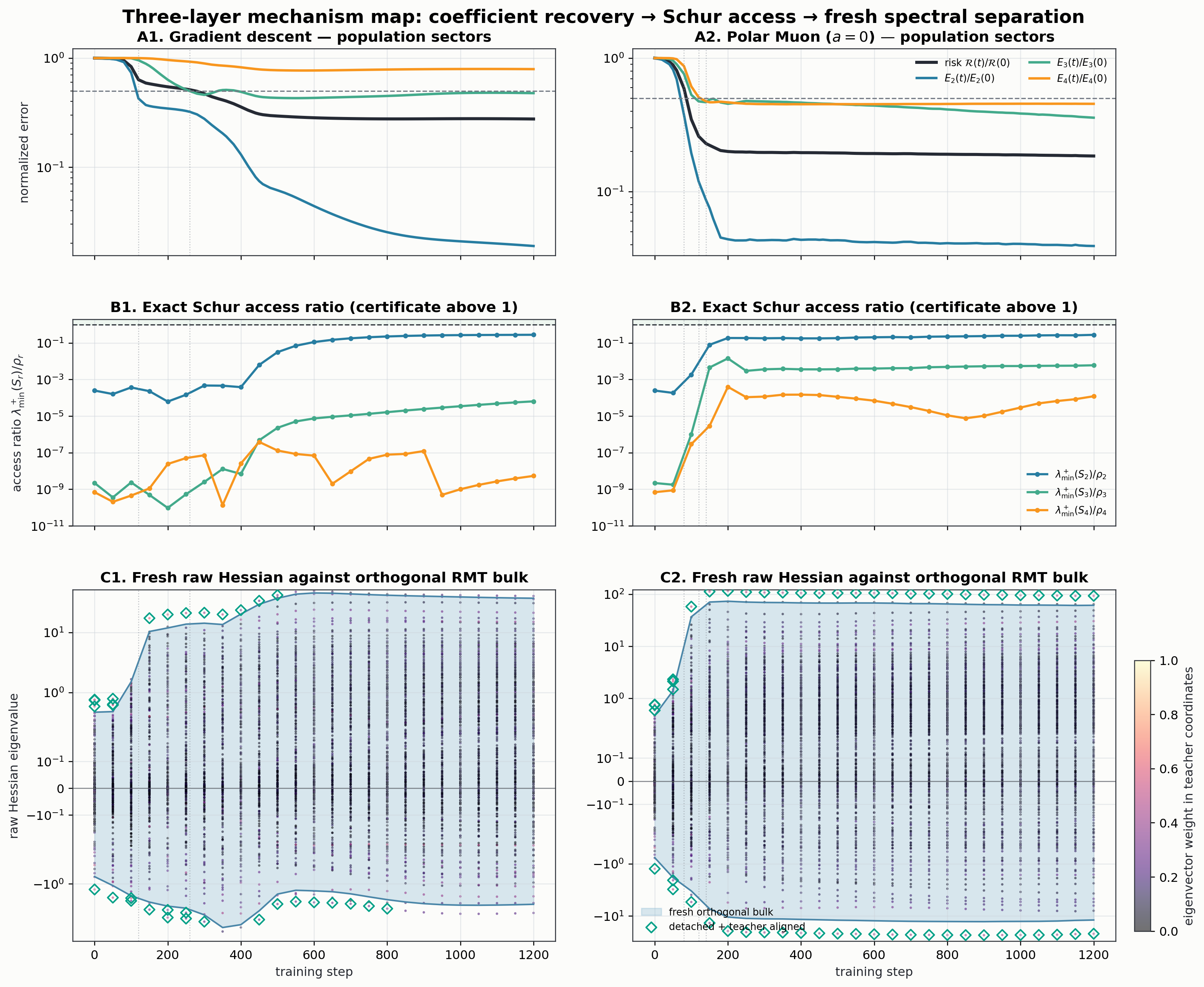
Row A: what is being learned

The horizontal axis is the full-batch training step. Black is exact population risk divided by its initial value. Blue, green, and orange are the degree-2, degree-3, and degree-4 Hermite errors, also normalized at initialization. The gray dashed level is one half. Vertical dotted lines mark the first recorded crossing of that level by each sector.

On this instance, gradient descent reaches degree 2 at step 120 and degree 3 at step 260; degree 4 is not reached by step 1,200. Polar Muon reaches the three events at steps 80, 120, and 140. These are trajectory facts for one shared instance, not an optimizer-ranking theorem. The separate twenty-pair confirmation finds no terminal-risk dominance.

Row B: whether the simple curvature certificate explains it

The ordinate is

\[\frac{\lambda_{\min}^+(S_r)}{\rho_r}\]

on a logarithmic scale. A value above one would certify positive curvature on the complete residualized degree-$r$ tangent space. Every displayed ratio is below one. The largest degree-2 value is about $0.28$ for both methods; the higher-order ratios are smaller.

Therefore this plot does not show that the Schur certificate proves the sector crossings. It shows the opposite: learning occurs while the sufficient bound remains inconclusive. The remaining candidates are conservativeness of the operator-norm residual bound, substantial cross-sector forcing, or both.

Row C: what the fresh Hessian sees

Every small point is an eigenvalue of the raw direct-weight Hessian built from one independent Gaussian probe. The blue band is the empirical spectrum of the orthogonal-coordinate block from the same probe. Point color is the eigenvector weight in teacher coordinates. Green diamonds satisfy both a fixed outside-bulk tolerance and a prespecified teacher-overlap threshold.

Under gradient descent, the number of marked modes falls from four at initialization to zero after step 850. Under polar Muon it settles at two from step 100 onward. This is persistent finite-size spectral separation. It is not yet a BBP theorem because the plot does not prove a limiting edge, track a unique eigenvalue branch, or control the same-data dependence.

What is in the public research package

• The journal PDF contains the model, theorem statements, proofs, conditional closure, and experiment.
• The TeX source bundle is the complete compilation source, including figures and bibliography.
• The claim ledger assigns every major statement to proved, imported, conditional, or empirical status.
• The literature and proof-interface map explains exactly what is imported from depth, DMFT, RMT, BBP, Kac–Rice, cavity, replica, AMP, and Muon—and what is not.
• The main experiment contains the paired training campaign, exact spectral update, fresh block-Wishart lift, and the tested Fréchet action.
• The dense-panel source reruns training and constructs all exact and spectral diagnostics.
• The exact sector-geometry table contains Schur ranks, eigenvalues, residual radii, projected Hessian minima, and cross-sector drift norms at every spectral checkpoint.
• The complete eigenpair table contains every plotted eigenvalue and teacher weight.
• The protocol report defines the common-probe coupling and every visual threshold.
• The algebra tests check the analytic link Hessian, finite-Gram Muon identity, strict descent, Fréchet derivative, block-Wishart projection, censored statistics, and exact sector geometry.

The theory article develops the deterministic and random-matrix reduction. The empirical article gives the paired confirmation, censored sector clocks, and sample-size campaign.

The theorem frontier

A full dynamic theorem now has a concrete checklist:

1. derive and prove the causal reused-data DMFT for the coupled trainable blocks;
2. prove a time-uniform block-Wishart global law and regular moving edges;
3. prove an anisotropic local law for the finite teacher-sector resolvent;
4. remove polynomial truncation or identify the separate extreme-observation spectrum;
5. prove a dynamic leave-one-out estimate for a Hessian built from reused observations;
6. take growing latent rank with a declared feature-strength law before claiming a universal scaling exponent;
7. derive the matrix-valued long-memory Onsager kernel and prove spectral-AMP state evolution;
8. derive the three-layer Kac–Rice complexity after gauge fixing and conditioning on representation invariants;
9. determine the edge exponent and Schur contact order before classifying a branch as continuous, discontinuous, or transient.

Until these locks are closed, the right formulation is a master reduction with exact interfaces and falsifiable diagnostics—not a general solved theory of all three-layer models.