Hierarchical three-layer learning
Does Muon Help a Hierarchical Three-Layer Model?
The empirical article. The companion theory map defines the exact three-layer Hermite model and separates deterministic dynamics, DMFT, and block-Wishart BBP statements. This page concentrates on what the experiments actually show.
Short answer
Muon helps on this pilot, but it does not win uniformly.
Across three paired training problems, exact polar Muon reaches a median exact population risk of $0.0871$, compared with $0.7569$ for gradient descent. A normalized $a=1/3$ spectral update reaches $0.0889$. Every spectral method beats gradient descent on two of the three pairs, but some transferred powers fail badly on the third pair.
The most stable qualitative result is not the optimizer ranking. It is the hierarchy: order-2 and order-3 Hermite sectors move early, while order 4 is the late bottleneck. Muon substantially changes the time at which that late sector becomes accessible.
These are reproducible finite experiments, not a universal scaling law or optimizer theorem.
A paired protocol designed to expose failures
The base configuration is
k=p=q=3, untied U/V, exact Gauss--Hermite test risk,
teacher sectors 2+3+4 with diagonal and mixed terms,
1,024 training samples, 1,200 full-batch steps,
3 paired repetitions, ambient d=32,
fresh Hessian sample n=145, orthogonal dimension 29.
Within each repetition, all four optimizers receive the same initialization and the same training set. The comparison is therefore paired rather than an average over unrelated problems.
The four update rules are:
- ordinary gradient descent;
- exact polar Muon, $a=0$;
- a transferred spectral power $a=1/7$;
- a normalized-branch comparator $a=1/3$.
Only the matrix blocks $V,U,A$ use the spectral transform. Biases and readout vectors retain gradient descent. Learning rates were stabilized in pilot runs, but the campaign is not a compute-matched hyperparameter tournament.
Most importantly, the reported test risk is evaluated by exact population Gauss–Hermite quadrature. It is not the finite training loss.
Training risk and sequential feature recovery
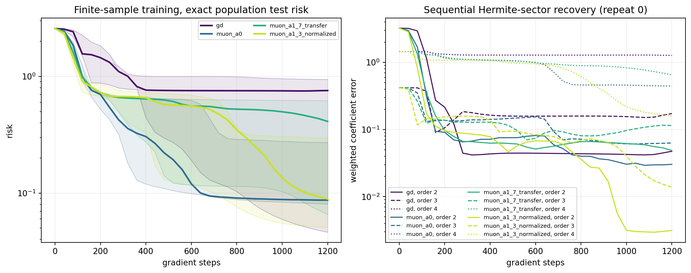
The endpoint risks are:
| optimizer | three paired endpoint risks | mean | median | wins vs GD |
|---|---|---|---|---|
| GD | 0.7569, 0.9416, 0.04620 | 0.5816 | 0.7569 | baseline |
| polar Muon $a=0$ | 0.2712, 0.08062, 0.08712 | 0.1463 | 0.08712 | 2/3 |
| transferred $a=1/7$ | 0.4114, 0.06553, 0.6195 | 0.3655 | 0.4114 | 2/3 |
| normalized $a=1/3$ | 0.08887, 0.05081, 0.2975 | 0.1457 | 0.08887 | 2/3 |
The paired ratios to gradient descent are revealing:
polar Muon:  0.358, 0.0856, 1.886
a = 1/7:     0.544, 0.0696, 13.41
a = 1/3:     0.117, 0.0540, 6.438
On the third pair, gradient descent happens to find a very low-risk solution and all three spectral rules do worse. The failure is extreme for the transferred powers. This rules out the naive conclusion that a single phase-retrieval exponent should be copied into every layer of the hierarchical model.
The clearest hierarchy signal
For repeat zero, define the half-error time of sector $r$ as the first checkpoint where its weighted coefficient error falls below half its initial value.
| optimizer | order 2 | order 3 | order 4 |
|---|---|---|---|
| GD | 120 | 160 | not reached by 1,200 |
| polar Muon $a=0$ | 120 | 120 | 680 |
| transferred $a=1/7$ | 80 | 120 | 1,160 |
| normalized $a=1/3$ | 80 | 80 | 800 |
Every method accesses lower orders first. The distinguishing event is the order-4 sector: gradient descent never halves it during the run, while polar Muon does so at step 680 and $a=1/3$ at step 800.
This supports the mechanism proposed by Dandi et al., the staged three-layer analyses of Nichani, Damian, and Lee and Wang, Nichani, and Lee, and the sequential-recovery viewpoint of Wortsman-Zurich et al.. It does not transfer their theorems to joint Muon training.
What happens when sample size grows
A second campaign uses five paired repetitions and nested data sets
\[n\in\{64,128,256,512,1024,2048\},\]with 800 steps per run. Nesting means that the $n=128$ data set contains the $n=64$ one, and so on. This reduces irrelevant variation when following a problem across sample sizes.
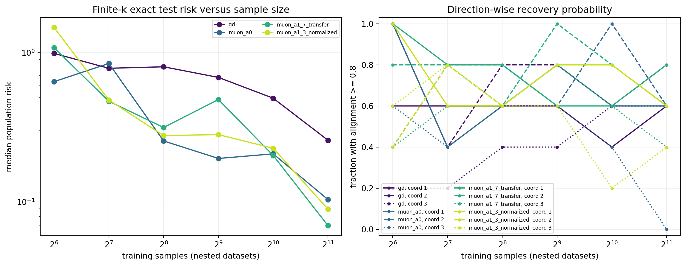
At $n=2048$, the median exact population risks are:
| optimizer | median risk | descriptive log–log tail slope |
|---|---|---|
| GD | 0.2592 | -0.536 |
| polar Muon $a=0$ | 0.1038 | -0.381 |
| transferred $a=1/7$ | 0.06948 | -0.779 |
| normalized $a=1/3$ | 0.08954 | -0.521 |
The slopes use only the four largest sample sizes. They are descriptive summaries of this fixed-$k$ experiment, not estimates of the growing-rank exponent in the sequential-feature-recovery theory.
The final-to-initial sector-error ratios at $n=2048$ are more stable:
| optimizer | order 2 | order 3 | order 4 |
|---|---|---|---|
| GD | 0.00971 | 0.327 | 0.302 |
| polar Muon $a=0$ | 0.00214 | 0.0985 | 0.106 |
| transferred $a=1/7$ | 0.000775 | 0.0981 | 0.0747 |
| normalized $a=1/3$ | 0.00266 | 0.168 | 0.0887 |
All methods reduce the quadratic sector strongly. The larger separation appears in orders 3 and 4, where the spectral methods leave substantially less residual coefficient error than gradient descent.
The direction-wise recovery frequencies are not monotone in $n$ with only five runs. One should therefore distinguish the robust risk/sector evidence from the noisier claim that each individual teacher direction undergoes an ordered sharp transition.
Fresh-sample Hessian spectra
At steps 0, 400, 800, and 1,200, the trained reduced state is lifted into an ambient Gaussian model and probed with fresh observations. Fresh probes matter: their orthogonal coordinates are independent of the finite block weights, so the orthogonal Hessian is exactly block-Wishart conditional on the reduced state.
The bulk interval is computed with the variational formula of Montanari and Saeed. A full eigenvector is called informative only if it lies outside the empirical orthogonal bulk and overlaps the teacher subspace.
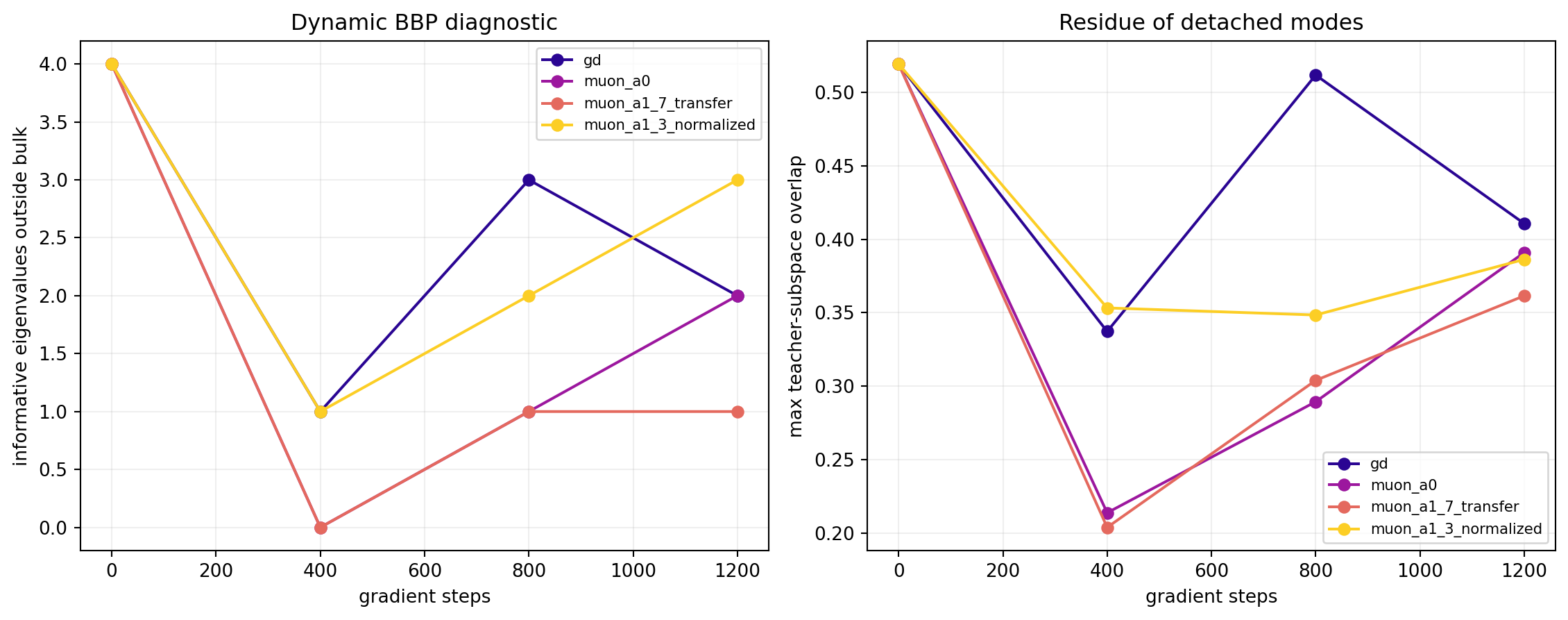
The raw counts of informative eigenvalues outside the empirical bulk are
                   step 0 → 400 → 800 → 1,200
GD                       4 →   1 →   3 → 2
polar Muon               4 →   0 →   1 → 2
a = 1/7                  4 →   0 →   1 → 1
a = 1/3                  4 →   1 →   2 → 3
The count is not monotone in training time. Branches can meet the bulk, re-emerge, or exchange spectral order. A dynamic BBP theory should follow branch identities and eigenvector residues, not only the largest eigenvalue.
Why rare samples cannot be ignored
The polynomial activation makes the Hessian block weights unbounded. To compare with the bounded block-Wishart theorem, the experiment clips block eigenvalues at 100 and records both clipped and raw results.
Across the recorded checkpoints, the median clipping fraction is about $2.1\%$ and the maximum is $6.2\%$. Despite this small fraction, the median operator-norm difference between raw and clipped full Hessians is about $32.9$. Rare Gaussian samples therefore have a disproportionate effect on spectral extremes.
This is why the blog and code keep two columns rather than presenting one misleading “theoretical edge”:
- clipped variational and clipped empirical bulk edges test the bounded theorem-facing object;
- raw empirical edges and eigenpairs describe the actual polynomial model.
A theorem for raw detached branches still needs tail control, an anisotropic local law, and a finite Schur argument. A same-data theorem additionally needs leave-one-out control because training and Hessian formation would reuse the same observations.
What was checked in code
Three focused algebra tests pass:
- the analytic preactivation Hessian matches automatic differentiation to about $10^{-16}$;
- the orthogonal Hessian projection matches the explicit block-Wishart construction exactly up to numerical precision;
- the SignSVD implementation has the intended singular-value action.
The complete training trajectories, fresh-sample spectral table, scaling runs, and JSON summaries are saved with the experiment rather than reconstructed from the plots.
What the evidence supports
The empirical conclusions are deliberately narrow:
- spectral updates can materially accelerate late high-order recovery in this hierarchical three-layer model;
- polar Muon and $a=1/3$ obtain much lower median endpoint risk than gradient descent on the three-pair pilot;
- no tested spectral rule dominates pairwise, so a universal transferred exponent is not supported;
- increasing sample size improves exact population risk, with clearer evidence in sector errors than in individual-direction thresholds;
- informative Hessian modes move relative to a block-Wishart bulk, but the present panel does not establish an asymptotic BBP crossing time;
- rare polynomial samples materially affect extreme eigenvalues even when only a few blocks are clipped.
The next decisive experiment
The next campaign should use at least 20 paired repetitions, jointly increase ambient dimension and latent rank, compare joint training with layerwise/frozen controls, sweep block-specific powers $(a_V,a_U,a_A)$, repeat every fresh spectral probe, and include a bounded smooth-link control. Only after those checks should held-out, cross-fit, and same-sample Hessians be compared.
Reproduce and inspect
- Main campaign: source, report, training trajectories, fresh-sample BBP table, and JSON summary
- Nested sample-size campaign: source, report, all runs, and JSON summary
- Algebra tests
- Complete scientific audit
- Theory companion
- Research-program map