This final part asks what changes during pretraining. The decoder is useful only if attention learns a better correction rule for PDE residuals. In linear-solver language, that correction rule is a preconditioner: a transformation that makes the hard directions of the linear system easier to solve.
The goal is to separate visual curve matching from mathematical proof. Some curves are exact identities, some are local diagnostics, and a global nonlinear training law for learnable-kernel attention would require replica-style order parameters.
There are three different kinds of training curve in the experiments, and they should not be confused.
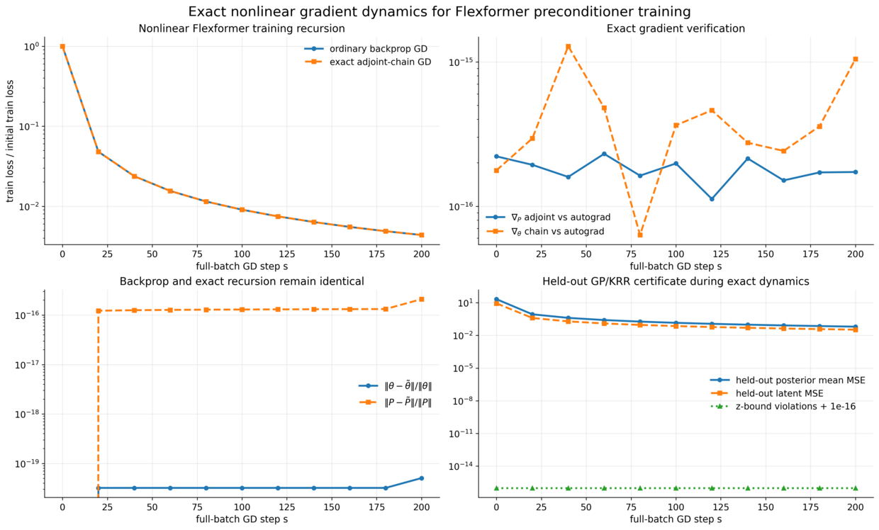
Compact diagnostic plots (simple experiments)
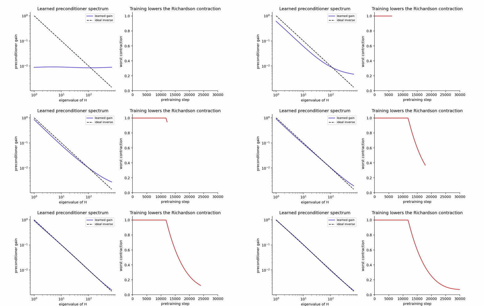 The animation shows a learned preconditioner moving toward the inverse spectrum of the task matrix. As the gain aligns with \(1/\lambda\), the worst Richardson contraction falls. This is the training-dynamics version of the solver story: pretraining is useful when it learns a better preconditioner, not merely a lower loss on stored tasks. 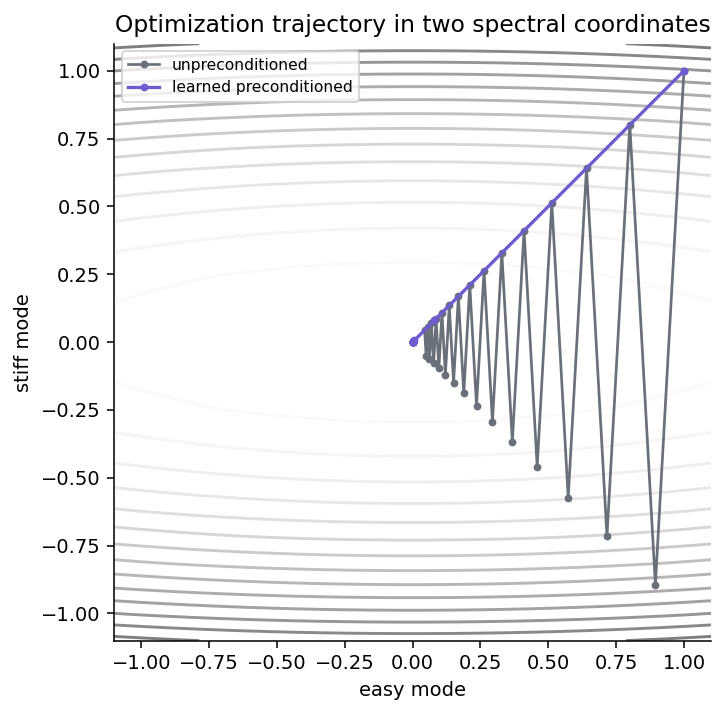 The phase portrait shows why conditioning matters. An unpreconditioned update zigzags across stiff directions, while a preconditioned update moves almost straight toward the solution. This is exactly the behavior the decoder should learn to reproduce in spectral coordinates. 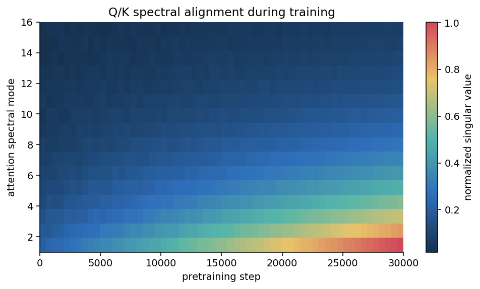 The heatmap tracks how attention modes become more structured during training. It is not a proof by itself, but it is the right diagnostic to pair with the theory: if query/key spectra align with useful residual directions, the value stream and feed-forward block can implement a stronger correction. 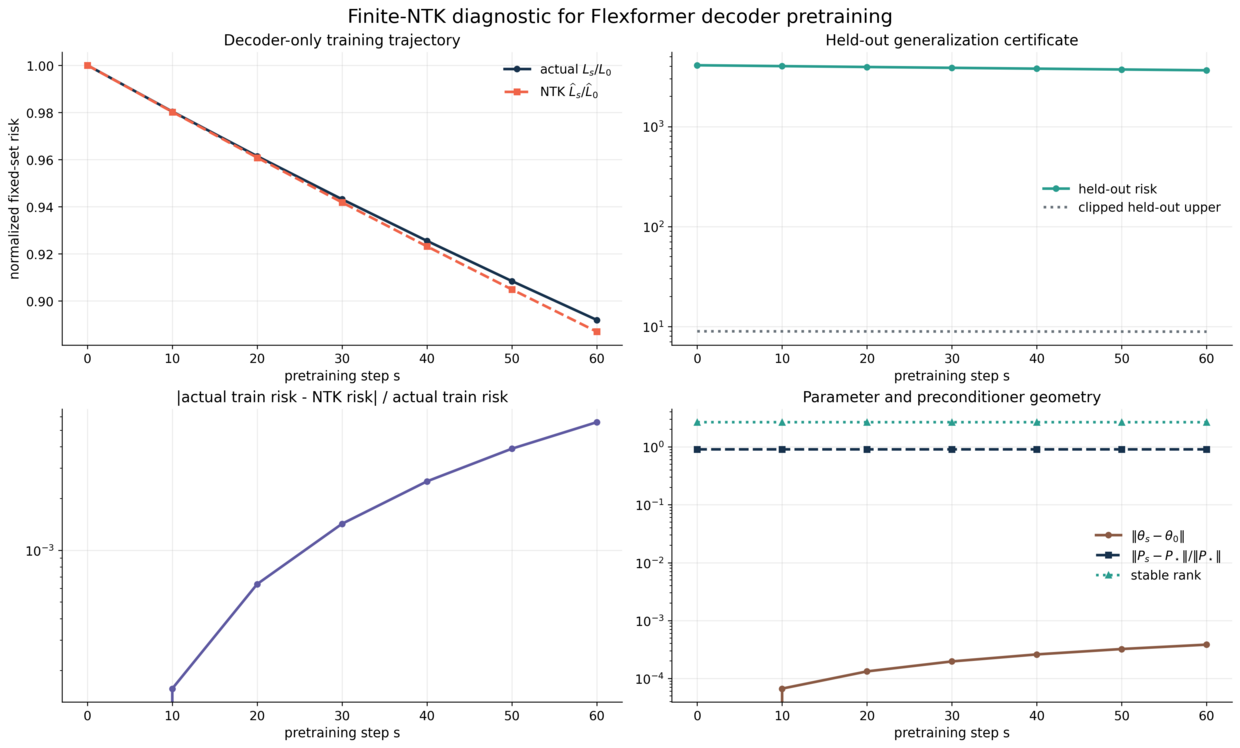 This is a local training prediction for the nonlinear decoder. It should be read as a finite-NTK diagnostic, not as the global replica law. 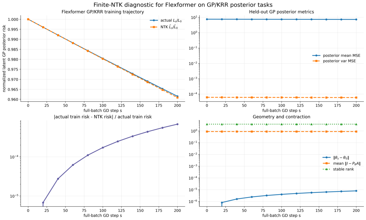 The GP/KRR run is the same local check after the posterior latent solve is used as the training target. It verifies that the local linearized curve can be very accurate in the lazy regime.The first is an exact population curve. For the encoder-only low-rank model,
\[G_s-G_\star=(G_0-G_\star)(I-\eta\Sigma_z)^s.\]This is a closed-form optimization trajectory. The plot compares online SGD against this exact curve, and the final observed/predicted risk ratio is
\[1.0005116697.\]The second kind is an exact frozen-checkpoint solver curve. Once a decoder preconditioner (P_\theta) is fixed,
\[e_L=(I-P_\theta H)^Le_0.\]This does not approximate the decoder. It is the decoder. That is why the reported Richardson bound violation rates are zero.
The third kind is a local training-dynamics curve for nonlinear learnable-kernel parameters. In the finite-NTK diagnostic,
\[r_s^{\rm NTK} = \left(I-\eta J_0J_0^\top/m\right)^s r_0.\]This predicts the training curve when the nonlinear model stays close to its initialization. The GP/KRR learnable-kernel run had relative curve error
\[6.83\times 10^{-4}.\]Finally, there is an exact finite-set nonlinear gradient recursion. For fixed training tasks,
\[\nabla_P\mathcal L_N(P_\theta) = \sum_{i=1}^N\sum_{\ell=0}^{L-1} \lambda_{i,\ell+1}r_{i,\ell}^\top,\]and
\[\theta_{s+1} = \theta_s-\eta DP_{\theta_s}^* \left[\nabla_P\mathcal L_N(P_{\theta_s})\right].\]The validation error against ordinary backprop was at machine precision:
\[\mathrm{relerr}(\nabla_\theta)=1.05\times 10^{-15}.\]So the correct reading is layered. The encoder-only curve is an exact closed population curve. The frozen decoder curve is an exact Richardson identity. The nonlinear learnable-kernel curve is a local NTK diagnostic. The finite training set calculation is an exact adjoint-gradient recursion.
The only thing not claimed is a scalar global replica closure for nonlinear learnable-kernel population training.
Why this distinction matters
It is tempting to look at a matching curve and say that the whole training theory is solved. That would be too fast. A curve can match for several different reasons.
For the encoder-only run, the match is a theorem about the population gradient flow of a quadratic objective. For the frozen decoder, the match is an algebraic identity. For the NTK diagnostic, the match says that the nonlinear model stayed in a local regime where the initial Jacobian remained predictive.
These are all useful, but they are not the same statement.
The finite-set adjoint recursion is the strongest nonlinear statement currently available in the experiments. It gives the exact gradient through all Richardson layers:
\[\lambda_{i,L}=\frac{z_{i,L}-z_i^\star}{NK}, \qquad \lambda_{i,\ell}=(I-P_\theta H_i)^\top\lambda_{i,\ell+1},\] \[\nabla_P\mathcal L_N = \sum_{i,\ell}\lambda_{i,\ell+1}r_{i,\ell}^\top.\]Then the learnable-kernel attention parameters update by the chain rule through (P_\theta). This is exact for the finite training set, but it is not a compact scalar population law. The state is the full parameter vector, or equivalently a high-dimensional set of overlaps between (P_\theta), the task matrices, and the residual covariance.
That is also why spectra alone are insufficient. Two preconditioners can have the same eigenvalues and singular values but different alignment with (H), and therefore different risk. Any replica-style closure must track mixed quantities such as
\[\operatorname{Tr}(PH),\qquad \operatorname{Tr}(PHPH),\qquad \operatorname{Tr}(PHS H^\top P^\top).\]The plots should therefore be read as a map of what is already exact and what is still structural. Encoder and frozen decoder dynamics are nailed down. Local learnable-kernel dynamics are well predicted. Global nonlinear population closure needs richer order parameters.
Reading the plots
The useful visual check is not just whether two curves are close. It is which two curves are close.
When the encoder held-out risk overlaps the exact population risk, that supports the low-rank recovery derivation. When actual decoder risk stays below the Richardson certificate, that supports the frozen optimization identity. When a finite-NTK prediction overlaps the nonlinear training loss, that supports the local linearization regime.
The exact-gradient plot adds another check: ordinary backpropagation and the hand-derived adjoint recursion produce the same parameter updates. The measured relative error in (\nabla_\theta) was about (10^{-15}), so the derivation is not merely plausible; it is numerically identical to automatic differentiation up to floating-point precision.
What would count as the next theory step?
The next step would be a closed population dynamics for the mixed overlap state, not just for the spectrum of (P_\theta). In a replica-style notation, that means tracking a joint law for the learned preconditioner, the task precision matrix, and the residual covariance. If that joint law closes under training, then the training curve could be predicted globally rather than locally.
Until then, the clean statement is layered: exact finite-set gradients, exact frozen-solver identities, accurate local NTK curves, and experimentally logged overlap dynamics.
External Papers Used
This series uses paper names only after introducing the problem they solve. The main external anchors are the following.
Low-rank in-context learning and replica theory. Kaito Takanami, Takashi Takahashi, and Yoshiyuki Kabashima, “Learning Linear Regression with Low-Rank Tasks In-Context,” arXiv:2510.04548. This is the reference for the high-dimensional low-rank task model and its replica generalization calculation.
Training dynamics of linear attention. Yedi Zhang, Aaditya K. Singh, Peter E. Latham, and Andrew Saxe, “Training Dynamics of In-Context Learning in Linear Attention,” arXiv:2501.16265. This is the reference point for exact gradient-flow phenomena in linear-attention ICL.
Learnable linear-attention kernels. Haoran Zhang and Feng Zhou, “Flexformer: Flexible Linear Transformer with Learnable Attention Kernel,” arXiv:2606.27748. This motivates the learned-kernel decoder experiments, but the posts distinguish local diagnostics from a proved global training theory.
Differentiable Galerkin assembly. Shizheng Wen, Mingyuan Chi, Tianwei Yu, Ben Moseley, Mike Yan Michelis, Pu Ren, Hao Sun, and Siddhartha Mishra, “Learning, Solving and Optimizing PDEs with TensorGalerkin,” arXiv:2602.05052. This is the relevant numerical-analysis reference for differentiable Galerkin assembly and PDE-constrained learning.