This post explains the data pipeline. The central move is simple: a transformer cannot directly manipulate continuous functions, so the PDE data are first represented by finite vectors. Once that is done, the prompt becomes a set of weak equations and the transformer decoder becomes a repeated solver step.
The figures are simple sanity checks for this geometry. They are here to make the construction visible; the proof questions come after the finite-dimensional objects have been fixed.
The methodology starts from one practical constraint: a transformer does not see functions directly. It sees finite-dimensional tokens. So the PDE is first projected into a Galerkin basis:
\[u(x)\approx \langle \mathbf u,\Phi(x)\rangle,\qquad f(x)\approx \langle \mathbf f,\Phi(x)\rangle.\]The PDE becomes
\[A\mathbf u=\mathbf f.\]If the task family has low-dimensional structure, the unknown object is a vector (z). It may parameterize the source,
\[f_z=f_0+\sum_k z_k^f\varphi_k,\]or the operator,
\[A(z^A)=A_0+\sum_k z_k^A A_k,\]or both. The prompt is then a collection of weak equations that identify (z). Abstractly,
\[G_mz\simeq b_m.\]The encoder estimates (z). The decoder solves the query problem after the task has been encoded.
Compact diagnostic plots (simple experiments)
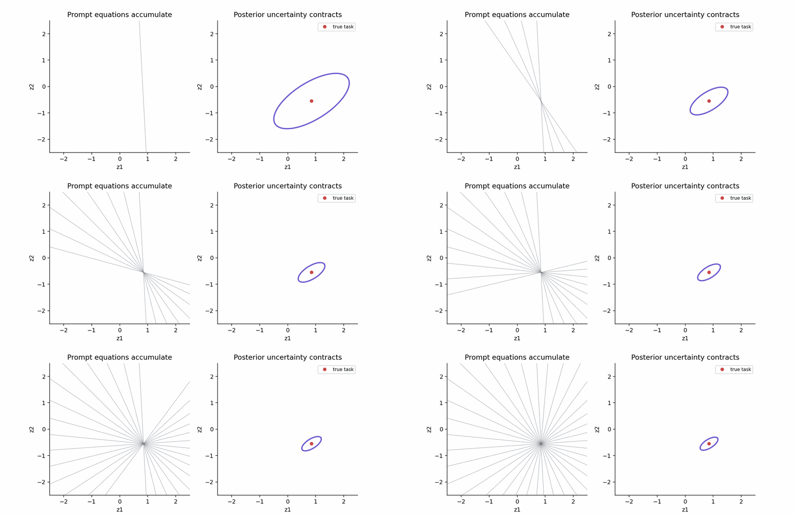 The animation is the algebraic core of the methodology. Each prompt pair adds weak equations, and the uncertainty over the latent task vector \(z\) shrinks. After this encoder step, the decoder is no longer solving an abstract problem; it is solving the query PDE attached to the inferred task. 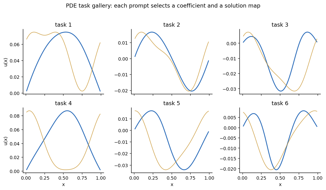 The gallery shows why the prompt has to be task-adaptive. Different coefficient fields produce different solution maps, even for smooth one-dimensional examples. A single fixed inverse is not enough once the operator itself moves. 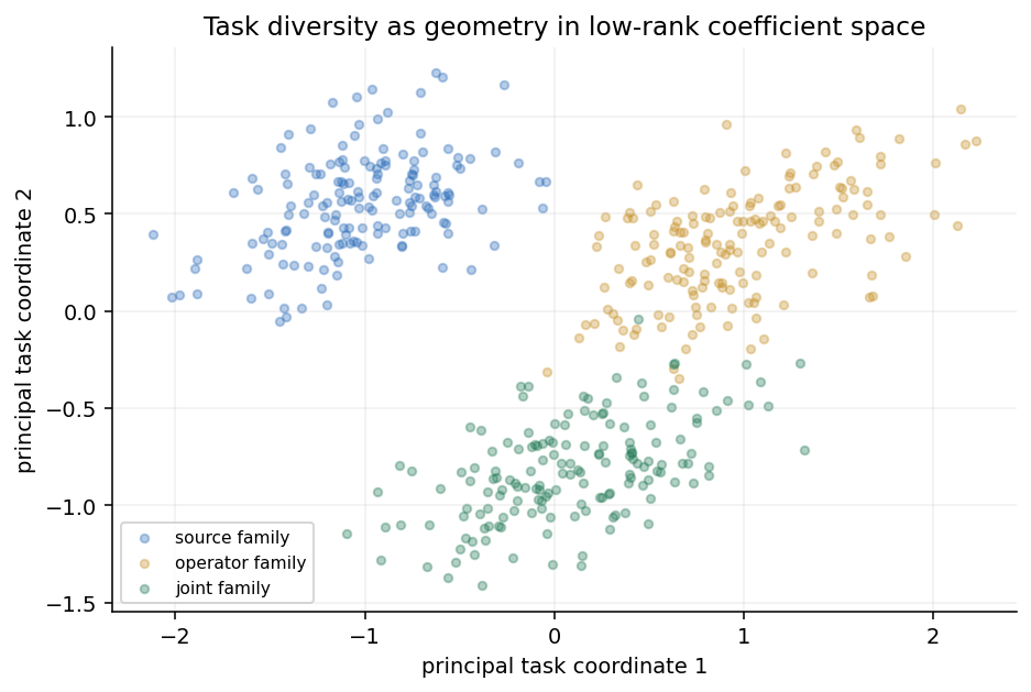 Task diversity is geometry in the latent coefficient space. Source-only tasks, operator-only tasks, and joint tasks occupy different regions. Training over many tasks should cover the directions that will later be inferred from a new prompt. 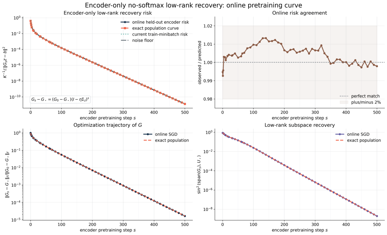 This plot is the encoder-only version of the methodology. Once the prompt has been turned into a finite matrix \(G_m\), population gradient descent has a closed risk curve. 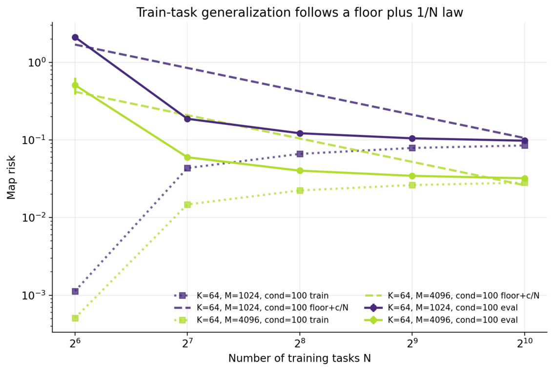 The train/eval comparison is the practical check that the finite-dimensional objects are not only fitted on stored prompts but transfer to held-out tasks.The transformer interpretation is:
- query/key scores route weak equations;
- values carry residual information;
- the feed-forward block implements a preconditioned correction.
For the latent least-squares system
\[H_m=G_m^\top G_m+\lambda I,\qquad c_m=G_m^\top b_m,\]the ideal recurrent update is
\[z^{\ell+1}=z^\ell+B_\Theta(c_m-H_mz^\ell).\]This is exactly a preconditioned Richardson iteration. The model is useful if the learned (B_\Theta) improves the contraction of the solve.
The experimental methodology isolates the moving parts. First test the abstract least-squares mechanism. Then test encoder-only recovery. Then test decoder-only preconditioning. Finally compose encoder and decoder in the Galerkin/PDE recast.
That is the main design choice: prove and test the algebraic mechanism before burying it inside a full PDE pipeline.
Three task types
There are three versions of the same idea.
In the source-coefficient version, the source has a low-dimensional expansion
\[f_z=f_0+\sum_k z_k^f\varphi_k.\]The prompt identifies (z^f), then the decoder solves the forward Galerkin system.
In the operator-coefficient version, the matrix itself is task-dependent:
\[A(z^A)=A_0+\sum_k z_k^A A_k.\]The prompt identifies (z^A), then the decoder solves the query equation with the reconstructed operator.
In the joint version, both source and operator coefficients are inferred. This is the most flexible case because it also covers rectangular, singular, or regularized systems:
\[\widehat u_\star = \arg\min_u \|A(\widehat z^A)u-f_{\widehat z^f,\star}\|^2+\gamma\|u\|^2.\]Why separate experiments are useful
A full PDE transformer experiment entangles too many effects: Galerkin error, operator identification, source identification, numerical conditioning, attention capacity, and decoder depth. The methodology here separates them.
First, test whether a recurrent decoder can behave like Richardson iteration. Second, test whether a low-rank encoder can recover a task subspace. Third, compose them. Fourth, insert the PDE weak-form encoder. This sequence makes failures interpretable.
For example, if the decoder fails in the constant-coefficient case, the problem is preconditioning or architecture capacity. If the decoder works but the variable-coefficient model fails, the problem is likely task identification. If both pieces work separately but not together, the issue is the interaction between encoder error and decoder stability.
The blog posts in this section follow that decomposition: constant coefficient, variable coefficient, proof details, focused bounds, and optimization trajectories.
Why KRR enters the story
The same algebra also covers finite-rank Gaussian-process regression. If
\[z\sim\mathcal N(0,\Lambda),\qquad f(x)=\phi(x)^\top z,\]then observing context values gives the posterior system
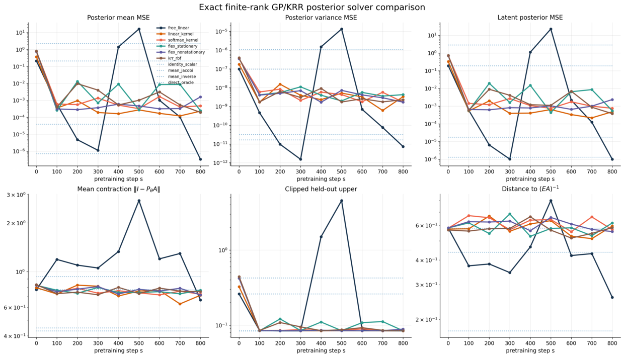
\[A z_{\rm post}=d, \qquad A=\Lambda^{-1}+\sigma^{-2}\Phi^\top\Phi, \qquad d=\sigma^{-2}\Phi^\top y.\]The KRR prediction identity is
\[\phi_q^\top z_{\rm post}=k_q^\top(K+\sigma^2I)^{-1}y.\]So a GP/KRR posterior mean can also be viewed as a latent linear solve. This is why the same decoder comparison can test free linear preconditioners, no-softmax linear attention, softmax attention, learnable-kernel linear attention, and KRR-like smoothers.
The point is not that every problem is secretly identical. The point is that the same recurrent solver primitive appears after the right finite-dimensional encoding. That is what makes a unified transformer-ICL methodology plausible: different front ends, same latent least-squares mechanics.
From proposal to experiments
The proposal describes the full PDE problem, but the experiments deliberately start with synthetic linear systems. That is not a retreat from the PDE setting; it is a way to remove Galerkin and discretization noise while testing the core mechanism.
The first experimental layer is decoder-only. Here the task system (Hx=d) is given directly. The only question is whether a learned attention block can act as a useful preconditioner. This isolates the solver.
The second layer is encoder-only. Here the model sees samples from a low-rank task distribution and must recover the latent representation. This isolates task identification.
The third layer is encoder plus decoder. The model first forms a latent task representation and then solves the induced system. This is the first place where the full error decomposition appears:
\[\text{end-to-end error} = \text{encoder floor} + \text{decoder error} + \text{interaction terms}.\]The fourth layer returns to the PDE setting. Weak-form equations produce the same (G_mz=b_m) encoder system, and the query solve becomes a Galerkin linear system. At this point, the synthetic algebra has become the PDE method again.
This ladder is the main methodological point. Each step has a falsifiable role. If the decoder-only step fails, the learned solver is not good enough. If encoder-only fails, the prompt is not identifying the task. If both work separately but not together, the issue is the stability of the composition. That makes the experiments interpretable rather than just numerical.
External Papers Used
This series uses paper names only after introducing the problem they solve. The main external anchors are the following.
Low-rank in-context learning and replica theory. Kaito Takanami, Takashi Takahashi, and Yoshiyuki Kabashima, “Learning Linear Regression with Low-Rank Tasks In-Context,” arXiv:2510.04548. This is the reference for the high-dimensional low-rank task model and its replica generalization calculation.
Training dynamics of linear attention. Yedi Zhang, Aaditya K. Singh, Peter E. Latham, and Andrew Saxe, “Training Dynamics of In-Context Learning in Linear Attention,” arXiv:2501.16265. This is the reference point for exact gradient-flow phenomena in linear-attention ICL.
Learnable linear-attention kernels. Haoran Zhang and Feng Zhou, “Flexformer: Flexible Linear Transformer with Learnable Attention Kernel,” arXiv:2606.27748. This motivates the learned-kernel decoder experiments, but the posts distinguish local diagnostics from a proved global training theory.
Differentiable Galerkin assembly. Shizheng Wen, Mingyuan Chi, Tianwei Yu, Ben Moseley, Mike Yan Michelis, Pu Ren, Hao Sun, and Siddhartha Mishra, “Learning, Solving and Optimizing PDEs with TensorGalerkin,” arXiv:2602.05052. This is the relevant numerical-analysis reference for differentiable Galerkin assembly and PDE-constrained learning.