Spectral transitions in multi-index models
When Does the Hessian Reveal a Hidden Direction?
Two versions of this work. This page explains the question and the conclusions without assuming random-matrix or Kac-Rice theory. The technical paper contains the full model, assumptions, proofs, and experiments.
The question in everyday language
A model can begin to learn a useful direction before that direction is clearly visible in a matrix computed from finite data.
This distinction is familiar outside machine learning. A weak radio signal may already carry a message, but a receiver cannot identify it until the signal rises above background noise. Here the message is a hidden teacher direction, the receiver is the empirical Hessian, and the background is a cloud of random eigenvalues.
The central question is:
When does a hidden direction become a separately detectable feature of the Hessian?
This article is about the Hessian geometry of multi-index phase retrieval. It is related to the Muon project because both study moving spectral transitions, but it is not a theorem about Muon and it is not a missing numbered part of the Muon series.
What the model is trying to learn
The target is a quadratic function built from several hidden directions. Each input $x$ is projected onto these directions, the projections are squared, and the results are combined with different strengths.
The student also uses several quadratic directions. During learning, its span can gradually align with the teacher span. We call this population capture: averaged over infinitely many fresh inputs, the student has acquired part of the hidden structure.
The empirical Hessian answers a different question. It is computed from finitely many observations and describes the local curvature of the observed loss. Random sampling fills most of its spectrum with a broad background. A teacher direction is spectrally visible only if it creates an eigenvalue outside that background and the corresponding eigenvector actually points toward the teacher.
What a BBP transition is
The dense background of eigenvalues is called the bulk. A structured signal can create an outlier, an isolated eigenvalue outside the bulk.
When the signal is too weak, the candidate eigenvalue remains absorbed in the bulk and its eigenvector is not reliably informative. As the signal becomes stronger, it reaches the bulk edge and separates. This threshold phenomenon is known as a BBP transition.
In a static problem the signal strength changes across experiments. In a learning problem the matrix itself changes with time, so both the bulk edge and the informative branch move. The transition is therefore dynamic.
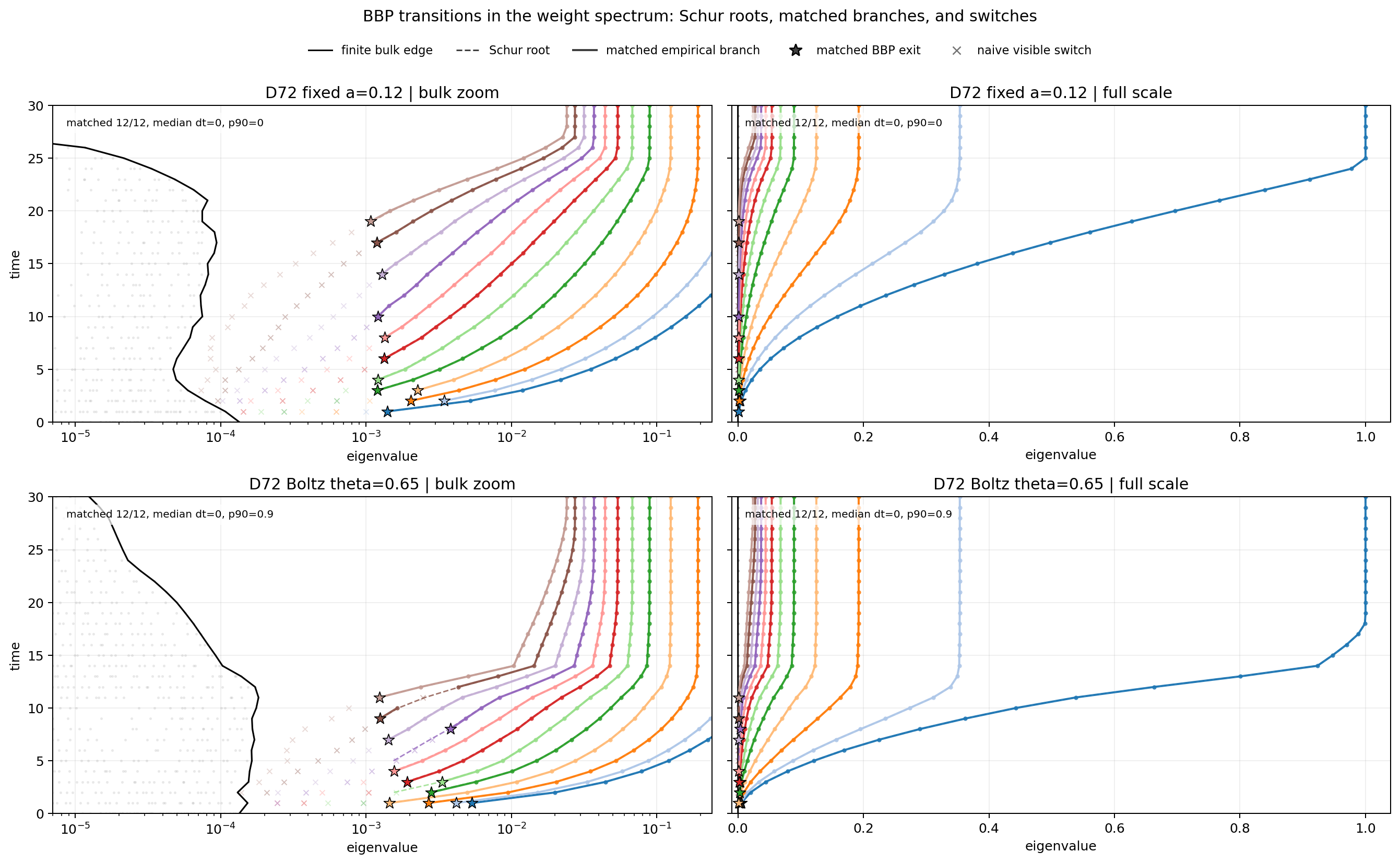
Time is vertical and eigenvalue is horizontal. The top row uses a fixed-power $D=72$ run with $a=0.12$; the bottom row uses the matched Boltzmann run with temperature parameter $0.65$. Left panels magnify the bulk edge and right panels show the full positive spectrum. The gray cloud is the empirical weight spectrum, the black curve is the finite bulk edge, colored dashed curves are Schur roots, and solid colored curves are the empirical branches matched by teacher residue. Stars mark matched exit events. Faint crosses are naive visibility switches that have not yet been assigned to the same Schur branch.
All 12 terminal roots are matched in each run. The median exit-time discrepancy is zero on the checkpoint grid; the 90th percentile is zero for the fixed run and $0.9$ checkpoint units for the Boltzmann run. This validates the branch-label algorithm in a fresh/frozen weight problem. It should not be cited as direct evidence for the Hessian law discussed in the surrounding section.
Why an isolated eigenvalue is not enough
An eigenvalue can be isolated for reasons unrelated to the teacher. The analysis therefore checks two conditions:
- the eigenvalue must lie outside the predicted random bulk;
- its eigenvector must have non-vanishing overlap with a hidden teacher direction.
The first condition concerns location. The second concerns meaning. The technical calculation uses a finite Schur complement to predict both the branch location and its teacher residue. In plain language, it removes the large random background and asks what remains in the small subspace carrying the structured signal.
This is also why following the largest or second-largest empirical eigenvalue can be misleading. Two informative branches may exchange their sorted order while retaining their teacher identities. The correct object to track is the labelled branch, not a fixed rank in a sorted list.
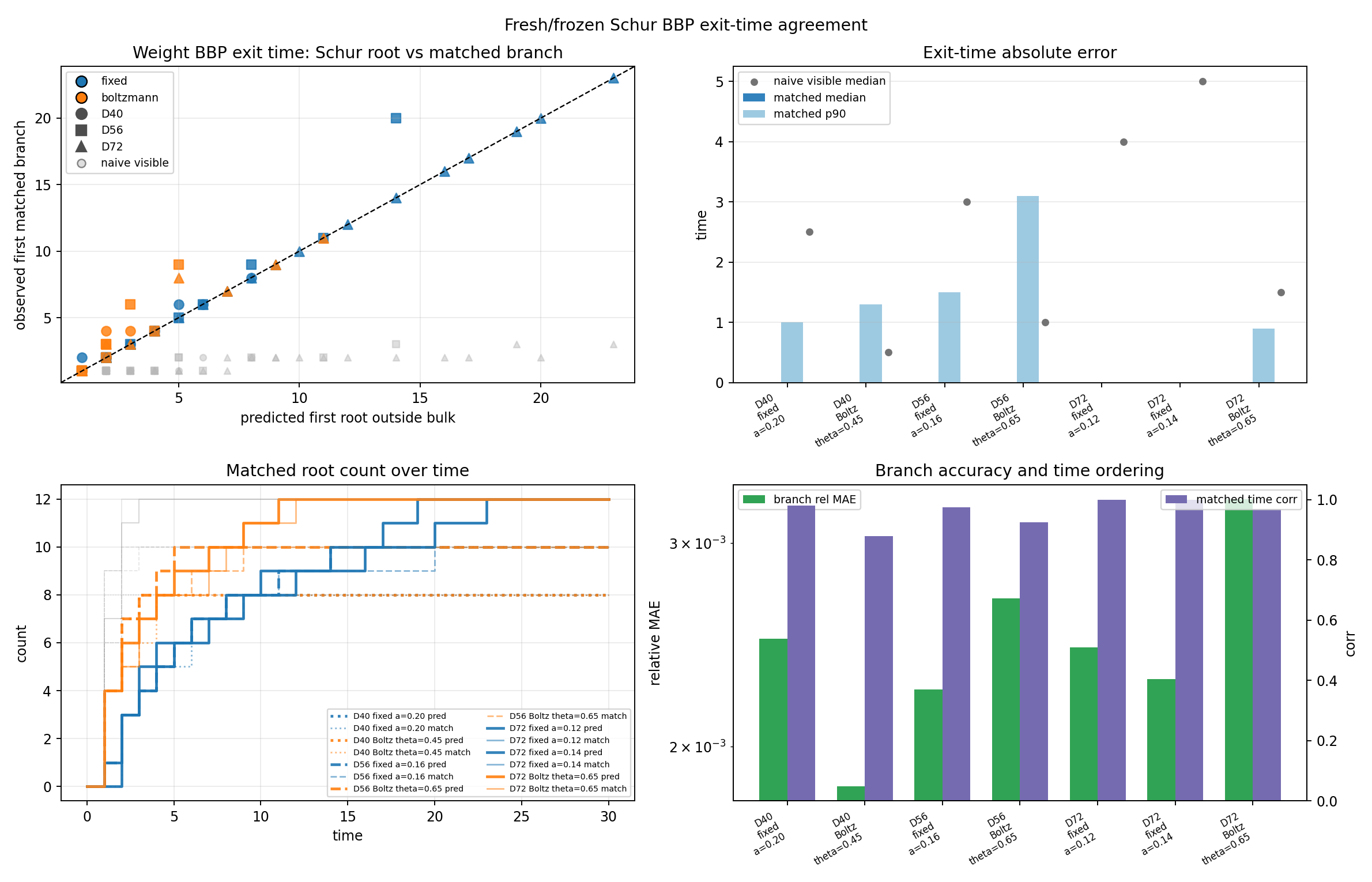
The upper-left panel compares the first predicted time outside the bulk (horizontal) with the first time the matched empirical branch is visible (vertical); marker shape identifies fixed and Boltzmann runs and the dashed line is equality. The upper-right panel reports absolute timing error for each run: black dots use naive first visibility, while blue bars summarize the matched branch. The lower-left panel compares the cumulative number of predicted and matched roots over time. The lower-right panel reports the relative branch-location error and time correlation.
Across 72 labelled branches, the matched median timing error is zero and its 90th percentile is one checkpoint; the median visible-branch relative eigenvalue error is $2.59\times10^{-3}$. Naive visibility has median timing error two and 90th percentile $9.9$. These numbers demonstrate why teacher labels are preferable to sorted rank. Again, this figure audits the matching machinery on fresh/frozen weight spectra; the Hessian contact calculation is a separate experiment.
Why the loss level matters
So far, the Hessian can be inspected along a prescribed learning trajectory. A second question asks about the entire loss landscape:
Among all critical points with a given loss value, what Hessian spectrum is typical?
The loss value is often called the energy. Low energy means a better fit. Different energy levels can contain different kinds of stationary points: minima, saddles, or highly unstable configurations.
Kac-Rice theory is a framework for counting and describing critical points under conditions such as fixed energy and zero gradient. The conditioning is important. Selecting points where the gradient vanishes changes the distribution of the data seen by the Hessian. One cannot automatically reuse the unconditioned Hessian law.
The multi-index setting is harder than repeating a one-direction calculation several times. The hidden directions interact through a matrix-valued state, and the conditioning acts jointly on all of them.
What the energy-resolved experiment checks
The technical construction first proposes a probability law for the finite set of relevant projections at a given energy. Once that law is supplied, a matrix Dyson equation predicts the bulk spectrum, and the same finite signal calculation predicts possible outliers and their teacher overlaps.
The numerical experiment tests this map at several energies. It compares the predicted density with independently generated finite Hessians.
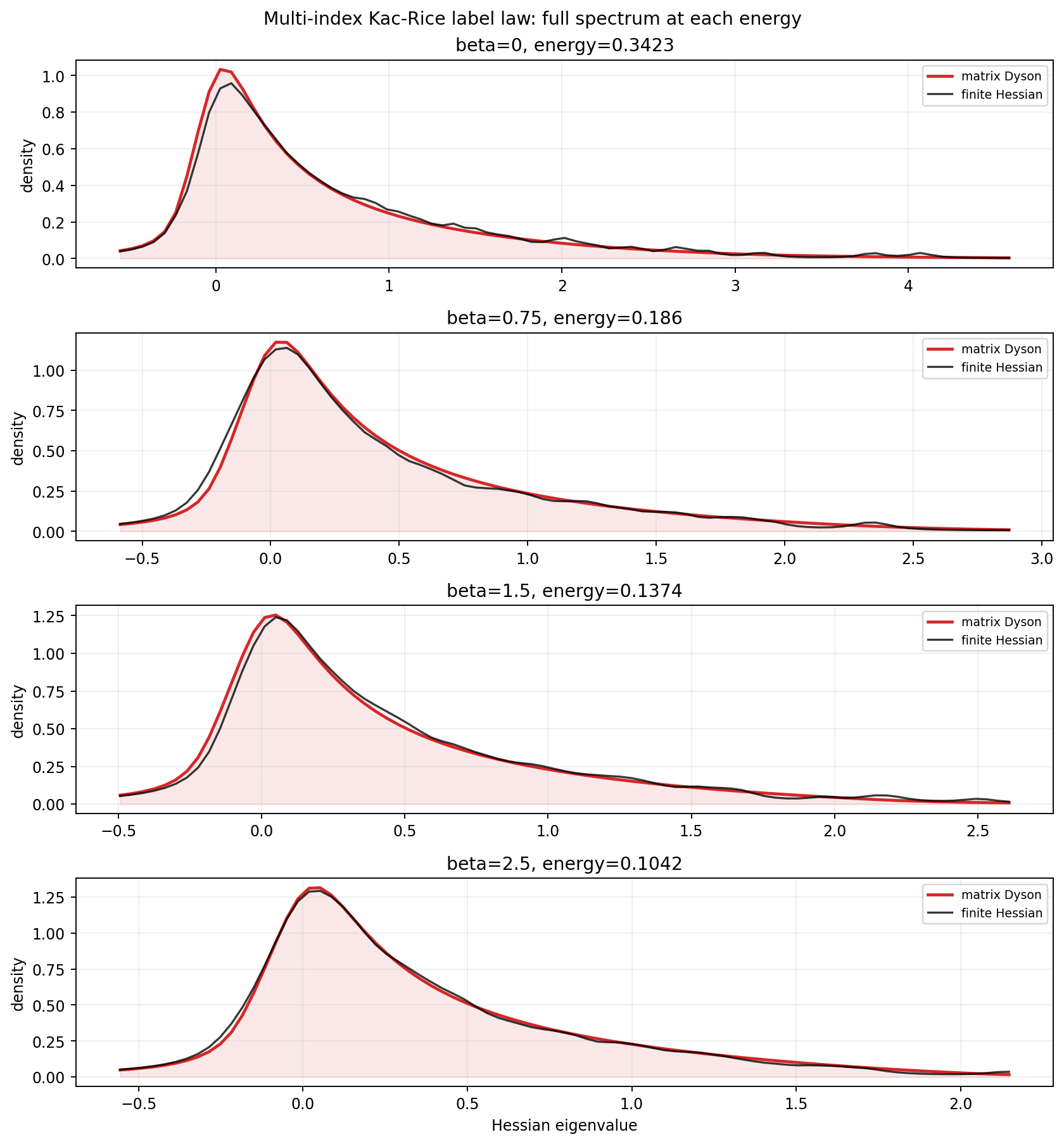
Each panel fixes one exponential energy tilt $\beta$; its attained energy is printed above the axis. The horizontal coordinate is the Hessian eigenvalue and the vertical coordinate is density. Red is the matrix-Dyson prediction computed from the candidate tilted projection law, while black is the density of independently generated finite Hessians. The experiment uses three student and three teacher modes, $d=54$, $n=162$, and the calibrated relative-loss offset $\kappa=0.35$. Across the four displayed energies, the largest relative $L^1$ density discrepancy is $0.0828$.
This agreement tests only the map from a supplied candidate conditioned law to a Hessian bulk. It does not prove that this law is the unique continuum Kac–Rice saddle, and it does not sample critical points directly from the original empirical landscape.
Mathematical scope
The population overlap equations and the finite signal–bulk decomposition are exact for the stated quadratic Gaussian model. For any fixed finite matrix, the exterior Schur determinant and the eigenvector residue used to label a branch are also exact identities.
For parameters independent of the Hessian sample, the bounded block-Wishart theory supplies a deterministic bulk after the regularity and aspect-ratio assumptions in the paper are imposed. Turning an exterior Schur root into a concentrating random eigenvalue additionally requires directional resolvent control; branch matching in the two weight figures above is a numerical audit, not that theorem.
The energy-conditioned conclusion is conditional on the proposed tilted finite-projection law. A complete Kac–Rice theorem still requires a continuum large-deviation principle for that law, determinant and index asymptotics, and a directional local law for the gradient-conditioned Hessian.
If the same data are used both to train the model and to form the Hessian, an additional trajectory-level leave-one-out argument is required. This same-data issue and the Kac-Rice conditioning issue are different proof obligations.
Takeaway
The original question was when a hidden direction becomes visible in the Hessian. Population learning alone does not answer it. Visibility occurs only when a teacher-labelled eigenvalue separates from the random bulk and its eigenvector retains teacher overlap. Along training this produces dynamic BBP transitions. Across the loss landscape, the same spectral test can be applied at fixed energy, but only after correctly accounting for the conditioning that defines a critical point.