Muon and controlled training dynamics
Muon for Phase Retrieval II: Choosing the Power During Training
Two versions of this work. This page explains the control idea without requiring optimal-control or random-matrix theory. The technical paper contains the mathematical model, derivations, and experiments.
The problem, recalled from the beginning
The teacher in this phase-retrieval model hides several directions. Some are strong and easy to learn; others are weak and appear only later. The first article showed that a fixed Muon power moves a learning front through this hierarchy.
A fixed setting is restrictive because training changes regime. Early in training, the most useful directions are strong and well separated from noise. Later, the remaining signal is weaker and closer to the random spectral background.
This article asks:
Should Muon use the same spectral power throughout training, or should the power adapt to what remains to be learned?
The proposed answer is a controller that observes a reduced description of training and chooses a power with both the present and the future in mind.
What the power controls
Muon transforms the singular values of the gradient. If a gradient direction has strength $\sigma$, the fixed-power family applies a response close to $\sigma^a$.
A smaller exponent flattens the spectrum. This gives weak directions more relative weight, but it can also amplify uncertain directions near the noise floor. A larger exponent is more conservative: it emphasizes directions that are already strong, but may take longer to reach the weak tail.
The best decision can therefore change with time. Early training may reward stability. Middle training may reward aggressive flattening. Late training may require another compromise as the remaining modes become dense and noisy.
What the controller observes
The controller does not need the full high-dimensional network state. It uses a reduced state containing quantities with direct meanings:
- how much of each teacher direction has been learned;
- how much signal remains;
- where the random spectral bulk begins and ends;
- how close each informative branch is to becoming visible;
- how previous updates continue to affect the current state.
This state is a model-based summary, not an extra neural network. Its purpose is to make the decision problem small enough to analyze.
A local decision is not enough
Suppose a very small exponent produces the largest immediate decrease in loss. It may still be a poor choice if it amplifies noise, distorts the next gradient, or delays a later spectral transition.
This is the same distinction faced by a route planner. The road that advances farthest during the next minute is not necessarily the road that reaches the destination first. A controller must attach a future cost to the current action.
In optimal-control language, the value function measures the best achievable future outcome from the current state. The Hamilton-Jacobi-Bellman, or HJB, equation expresses the consistency of that future value over time. The blog does not derive this equation; the technical paper does. The conceptual consequence is:
Choose the power that balances immediate spectral progress with the way today’s update changes tomorrow’s options.
Why a distribution over powers appears
Always selecting one exact minimizer can make the schedule unstable. Two nearby powers may have almost identical predicted costs, and small estimation errors can cause abrupt switching between them.
The relaxed controller instead assigns more probability to powers with lower predicted cost. Its distribution has the familiar Boltzmann form
\[\text{probability of }a \;\propto\; \exp\{-\beta\times\text{predicted cost of }a\}.\]The parameter $\beta$ controls decisiveness. A small $\beta$ spreads weight over several plausible powers; a large $\beta$ concentrates near the current minimizer. This smoothing is a deliberate regularization of the decision rule. It is not thermal noise added for visual effect.
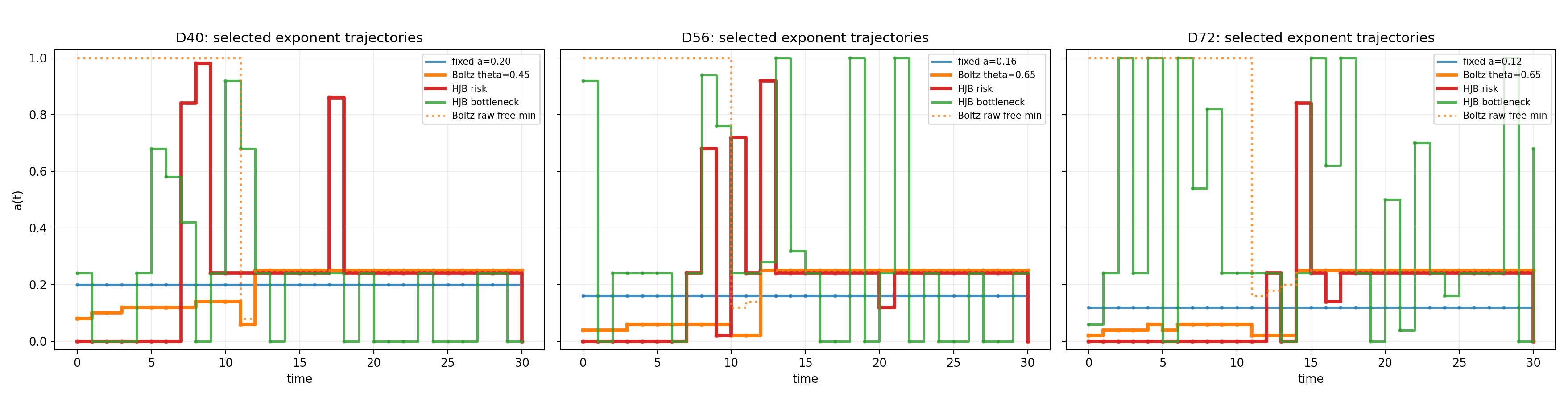
The three panels correspond to $D=40$, $56$, and $72$. Training time is horizontal and the selected exponent $a(t)\in[0,1]$ is vertical. Blue is the fixed baseline, orange is the entropy-regularized Boltzmann policy, red is the risk-terminal HJB policy, and green is the bottleneck-terminal HJB policy. Curves are drawn as step functions because the action is updated only at the recorded decision times. The dotted orange curve, when present, is the unregularized point minimizer before Gibbs averaging.
This is a collection of selected trajectories, not a statistical summary: there are no seed bands and the three dimensions use different fixed baselines. Smoothness of the orange path is induced by entropy regularization. It does not show that the barycentric action follows the same state equation as the randomized policy; that replacement additionally requires the small-curvature/variance bound stated in the technical paper.
The role of spectral denoising
There is also a purely local question: if the current gradient is a noisy matrix, which transformation best separates signal from noise right now?
Message-passing methods provide an idealized spectral denoiser for a specified probabilistic channel. Muon cannot implement an arbitrary denoising curve because it only has a one-parameter power family. The calculation therefore projects the unrestricted local denoiser onto the nearest useful Muon power over the currently active spectral range.
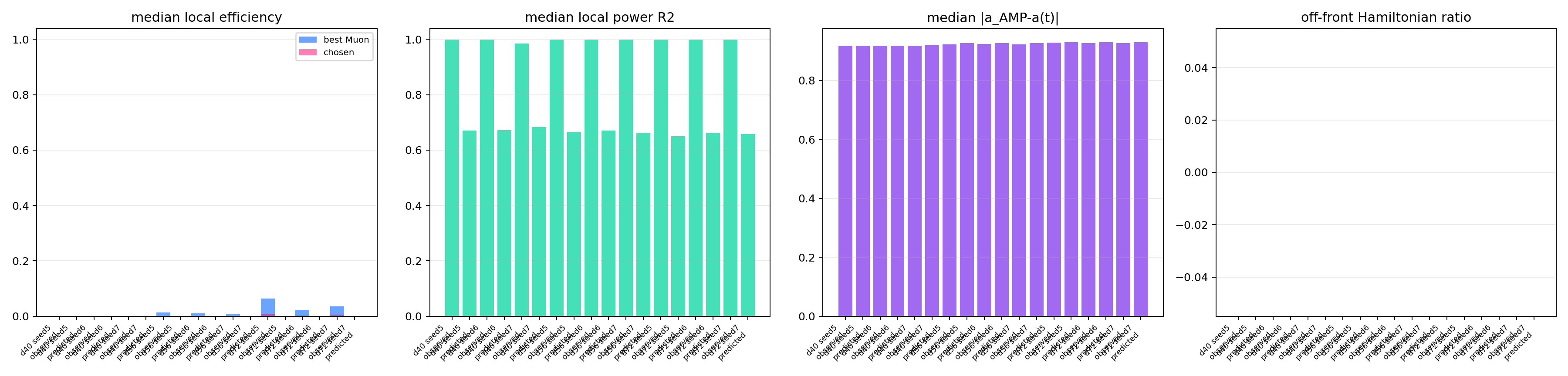
Each adjacent observed/predicted pair on the horizontal axis is one run at $D\in{40,56,72}$ and seeds 5–7. In the first panel, the blue bar is the best efficiency attained after restricting the likelihood-ratio benchmark to the one-parameter Muon power family; the pink bar is the efficiency at the action actually selected by the controller. Both are normalized by the unrestricted likelihood-ratio efficiency. The second panel is the $R^2$ of a local power-law fit to that likelihood ratio. The third is $|a_{\rm AMP}-a_{\rm chosen}|$. The fourth is the share of the Hamiltonian assigned outside the selected front.
For the observed signal channel, the local power fit is numerically excellent ($R^2$ is typically above $0.98$), but its median minimizer is $a_{\rm AMP}=1$, whereas the chosen exponents are about $0.07$–$0.09$. The median gap is therefore about $0.92$. For the predicted signal channel, the local $R^2$ is only about $0.65$–$0.68$. The plotted off-front ratio is zero by construction of these selected windows. The audit consequently rejects the strong interpretation that the implemented controller is the local AMP denoiser projected onto the Muon family.
The weaker statement remains valid: the unrestricted denoiser is a local benchmark, while the HJB action also includes future cost and may select a different exponent. The two complete algorithms are not equivalent, and this figure quantifies rather than hides that difference.
What changes in the spectrum
The objective is not merely a smoother loss curve. The controller tries to organize when teacher directions become separately visible.
A direction becomes spectrally visible when its informative eigenvalue leaves the random bulk. Because the power changes the update, it changes both the informative branch and the surrounding noise spectrum. The relevant target is therefore the future sequence of crossings, not just the largest eigenvalue at the current step.
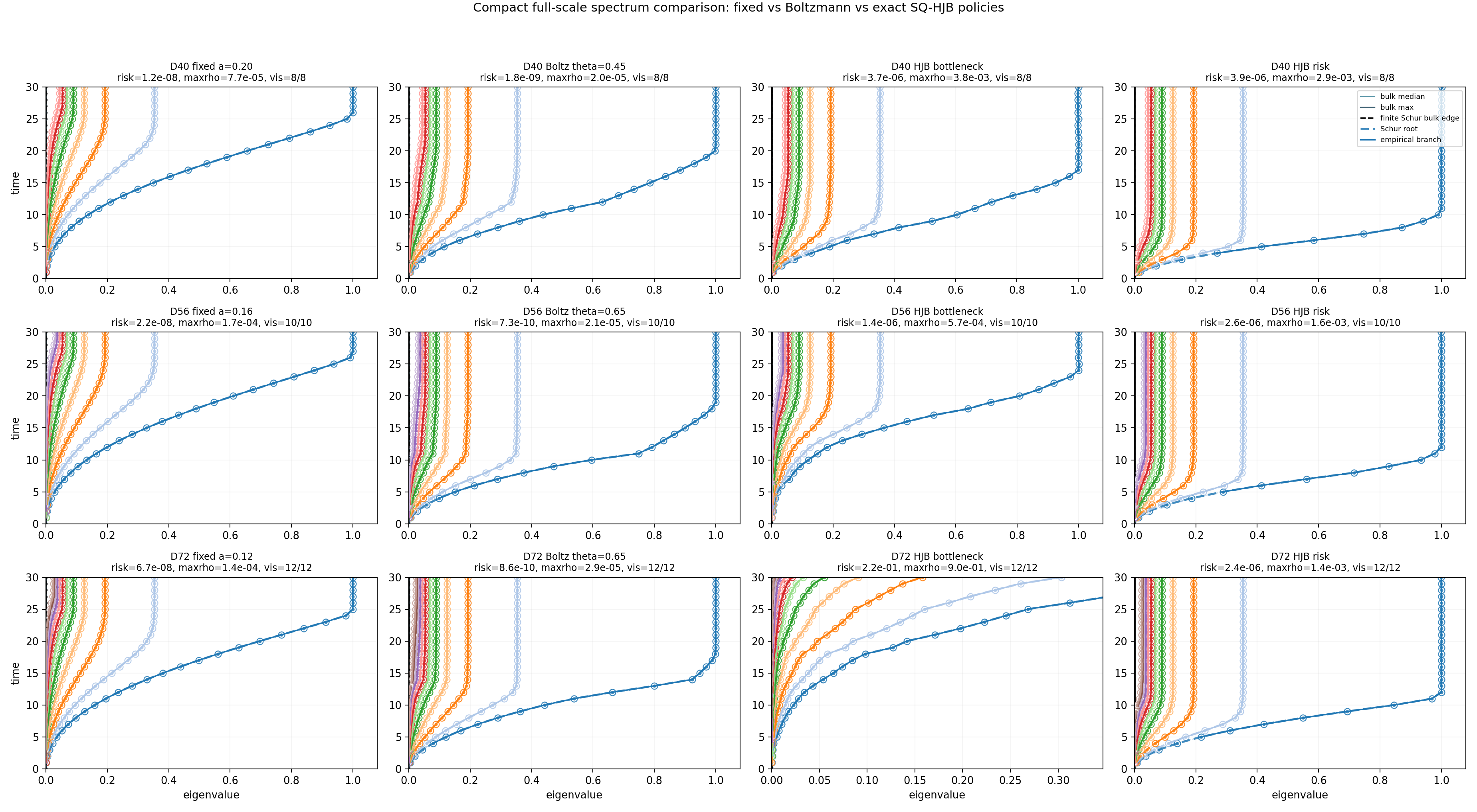
Rows correspond to $D=40$, $56$, and $72$; columns compare a fixed power, the Boltzmann controller, the bottleneck HJB controller, and the risk HJB controller. Time is vertical and weight eigenvalue is horizontal. The two thin curves nearest the origin track the median and maximum of the finite bulk; the dashed black curve is the finite-Schur bulk edge. For each teacher mode, the colored dashed curve is the finite Schur root and the colored solid curve with open circles is the residue-matched eigenvalue branch. Each title reports terminal population risk, the worst residual teacher fraction, and the number of visible roots.
All terminal roots are visible in these stored runs, but policy quality is not uniform. For example, the $D=72$ bottleneck-HJB run ends at population risk $0.218$, compared with $6.68\times10^{-8}$ for the fixed run and $8.65\times10^{-10}$ for the Boltzmann run. Moreover, the finite Schur roots and full eigenvalues come from the same frozen matrix; their near-machine agreement checks the implementation of the Schur identity. It does not test a deterministic high-dimensional outlier law or establish that an adaptive schedule improves risk.
Mathematical scope
For a specified reduced deterministic state equation, the sensitivity of the trajectory to a change in control, the backward adjoint, and the constrained stationarity conditions are exact. The Gibbs policy is the exact optimizer of the entropy-regularized action at a given reduced state. Replacing the randomized policy by its mean exponent is exact only for drift affine in $a$; otherwise the paper supplies an error bound involving action variance and $\partial_{aa}b$.
The local projection from an idealized denoiser to a Muon power is exact only under the stated channel model and active-window assumptions. It is not a proof that Muon reproduces the full message-passing state evolution.
The numerical bridge audit above does not satisfy the stronger projected-AMP interpretation for the implemented controller. Independently, the remaining probabilistic step from the fixed-power analysis persists: one must identify the reduced fresh-sample state with the stochastic trajectory when the same finite data are repeatedly reused.
Takeaway
The problem was to decide whether Muon’s spectral power should remain fixed while the learning task changes. The proposed controller says no: use the current learned masses and spectral margins to estimate immediate progress, add the future cost of changing the trajectory, and regularize the choice so that nearly equivalent powers do not cause unstable switching.
The final Muon article explains exactly which parts of this program are proved and which bridge is still open: What Is Proved and What Remains Open.