This experiment asks one concrete question: how should Muon rescale a matrix gradient when the target contains both strong and weak directions?
Standard Muon completely flattens the singular values of a matrix gradient. Adding a power creates a continuum between gradient descent and Muon, so the optimizer can change how much flattening it applies during training.
The experiment
The input $x$ is Gaussian. The target is a sum of squared projections,
\[y=\sum_{j=1}^{D}\lambda_j(\theta_j^\top x)^2,\]where the orthogonal directions $\theta_j$ are hidden and their strengths $\lambda_j$ decrease with $j$. Strong directions are easy to find; weak directions are progressively harder. This standard test problem is called multi-index phase retrieval.
The student is trained on this target with a matrix-valued gradient. If
\[G=U\,\mathrm{diag}(\sigma_1,\ldots,\sigma_r)V^\top,\]the update replaces each gradient singular value $\sigma_i$ by $\sigma_i^a$.
- $a=1$ is the ordinary matrix gradient.
- $a=0$ gives every nonzero singular direction equal size: the polar or SignSVD form of Muon.
- Values between zero and one interpolate between them.
A smaller exponent boosts weak gradient directions relative to strong ones. That can reveal weak signal sooner, but it can also boost noise. The experiment is therefore about choosing this exponent, not about claiming that the smallest value always wins.
Why the power may change
Early in training, large singular directions can contain reliable signal. Later, the useful information may be concentrated in smaller directions that ordinary gradient descent barely moves. The same amount of flattening need not suit both stages.
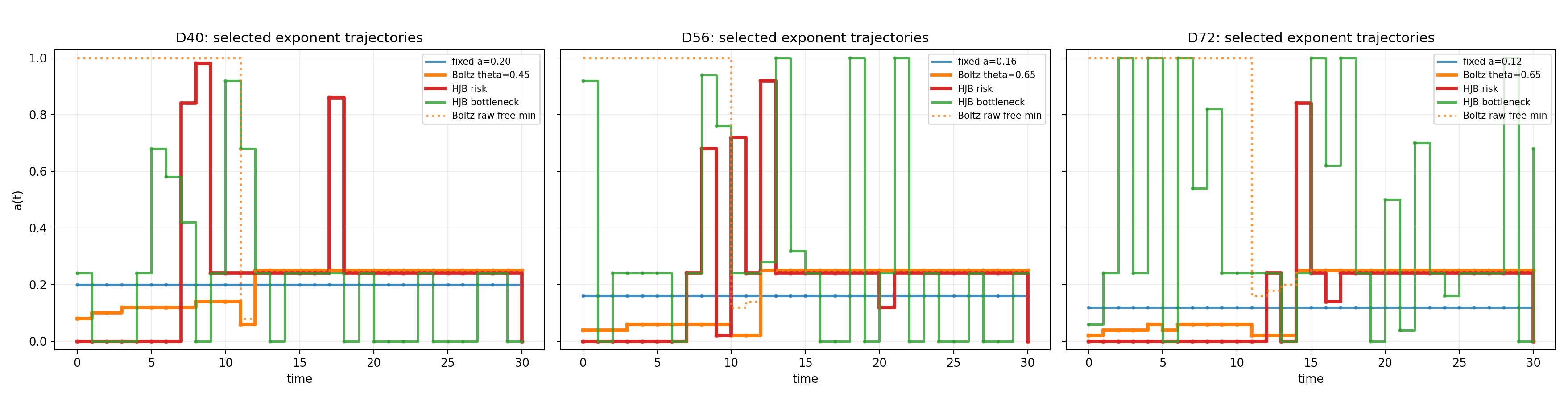
The plot below compares fixed powers with policies that change the power during training. Its purpose is to show that the preferred setting can move with the training state, not to advertise one universal numerical value.
The exponent chosen during training
Why a Boltzmann rule appears
At each checkpoint, the reduced model predicts the future cost of using each candidate exponent. Call that cost $C_t(a)$. Always taking the single lowest estimate is unstable when several exponents are nearly tied, so the controller assigns them probabilities:
\[\pi_t(a)=\frac{\exp[-\beta C_t(a)]} {\int_0^1\exp[-\beta C_t(u)]\,du}.\]This is simply a Gibbs or Boltzmann distribution over the available updates. A large $\beta$ concentrates on the currently predicted best exponent. A smaller $\beta$ averages over several plausible choices. The derivation comes from adding an entropy penalty to the finite-horizon control problem; the cost $C_t$ includes both the immediate loss decrease and how today’s update changes the remaining training path.
The important point is practical: the useful exponent can change because the problem changes during training. Early on, strong directions dominate. Later, only weaker and noisier directions remain.
Three views of the same run
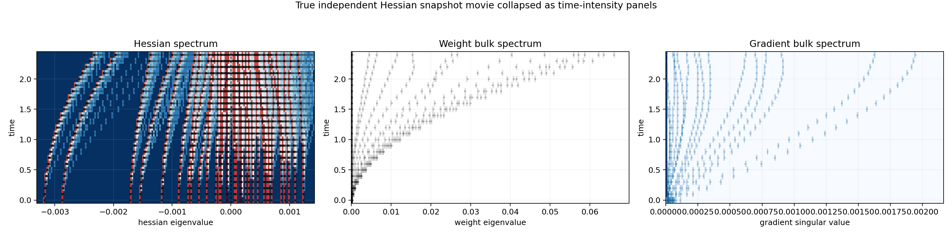
The experiment records three matrices at every checkpoint:
- Gradient: the update proposed at that moment.
- Weights: the directions accumulated by all earlier updates.
- Hessian: the local curvature of the loss.
Their eigenvalues are on different numerical scales, so the panels should not be compared left-to-right by magnitude. The point is temporal: structure becomes visible at different times in the three matrices.
Gradient, weights, and Hessian during one training run
What BBP means here
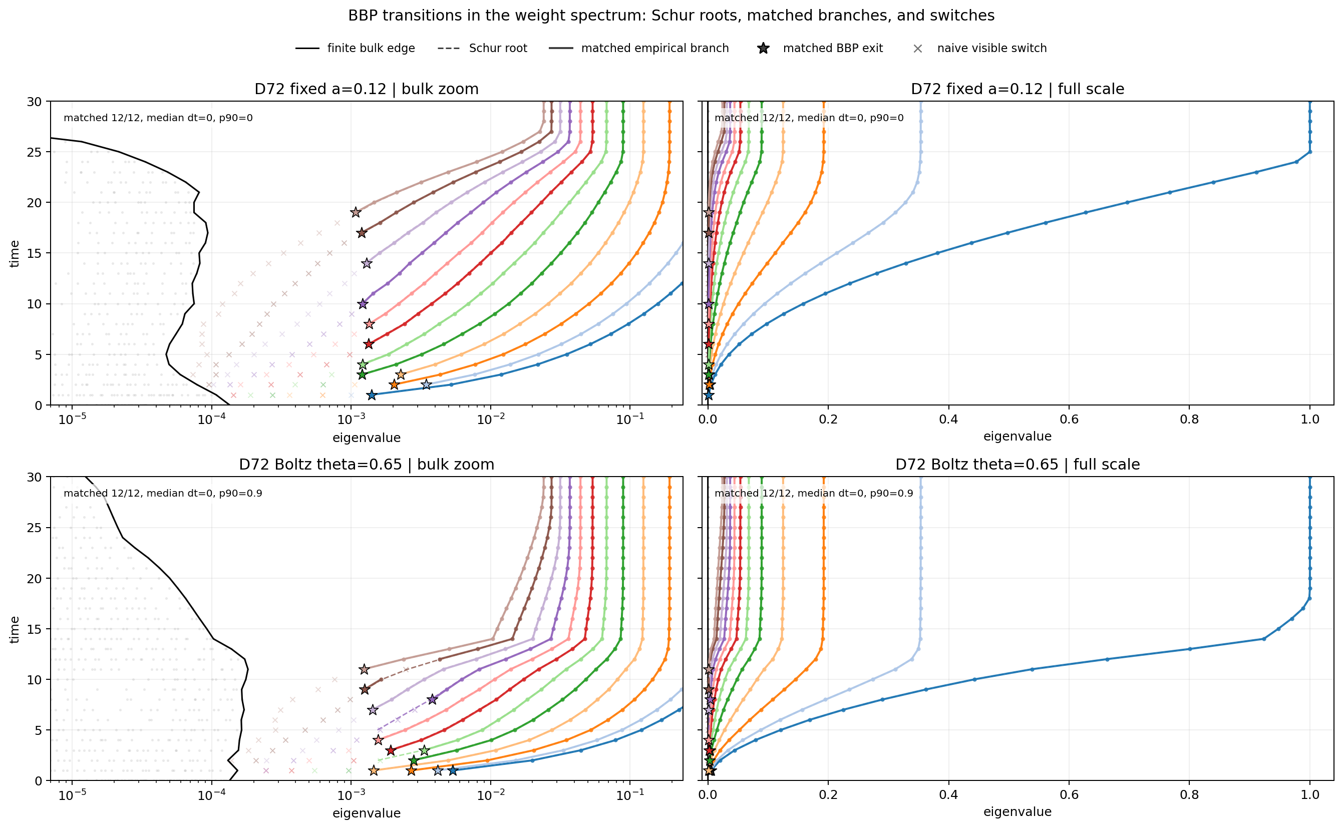
With finite data, most eigenvalues form a dense background cloud. A hidden direction becomes separately detectable when it produces an eigenvalue outside that cloud and the associated eigenvector aligns with the true direction. This separation is called a BBP transition, after the classical result of Baik, Ben Arous, and Peche.
The next plot tracks these events in the weight spectrum. Time is vertical. The black curve is the edge of the background spectrum. A colored line is one hidden direction. A star marks the checkpoint where that direction becomes an isolated, identifiable eigenvector.
When each hidden direction becomes detectable
What this shows
Adding the power $a$ turns Muon from one update rule into a family of update rules. The fixed experiments show that the best constant power depends on the size of the problem. The adaptive experiment goes one step further: it changes the power as training moves from strong directions to weak ones.
In this controlled problem, that adaptive choice beats the selected fixed-power baseline. The mechanism is visible in the plots: changing $a$ changes which singular directions receive a large update, and therefore when the hidden directions become detectable.
This is the claim of the post: a power inside Muon can be optimized as part of training, instead of being treated as a fixed design choice. The numerical values above belong to this phase-retrieval experiment; the broader proposal is to tune or control the power for the model being trained.
References and provenance
- Dong and Sawin, Muon$^p$: Muon with Fractional Spectral Powers introduces fractional spectral-power updates between Muon and gradient descent.
- Wu et al., DynMuon: A Dynamic Spectral Shaping View of Muon dynamically schedules the spectral power during language-model training.
- Paquette et al., Phases of Muon: When Muon Eclipses SignSGD gives a high-dimensional analysis of Muon/SignSVD and motivates studying spectral power laws.
- Baik, Ben Arous, and Peche, Phase Transition of the Largest Eigenvalue for Non-Null Complex Sample Covariance Matrices is the classical source of the BBP transition.
- Defilippis et al., Optimal Spectral Transitions in High-Dimensional Multi-Index Models studies optimal spectral recovery in the multi-index setting.
- The experiment code and numerical work are maintained in the research repository.