Muon and controlled training dynamics
Muon for Phase Retrieval III: What Is Proved and What Remains Open
Two versions of this work. This page is a non-technical proof map. It explains what each mathematical layer contributes and where the argument is still conditional. The main manuscript and full mathematical details are the expert versions.
The full problem, recalled
The model hides many directions with decreasing strengths. A student is trained by Muon, which changes the singular values of the gradient before updating the weights. The project aims to predict four things:
- how quickly each hidden direction is learned;
- when that direction becomes visible in a finite spectrum;
- how the gradient, weight, and Hessian spectra evolve together;
- how the Muon power should change during training.
These conclusions do not all have the same status. Some follow from exact algebra. Some use established random-matrix theorems after matching their assumptions. Some are supported by experiments but still need a new theorem.
The purpose of this post is to keep those layers separate.
Layer 1: exact finite-dimensional algebra
Although the weights live in a high-dimensional space, the quadratic population model only depends on overlaps among the student directions and the hidden teacher directions.
This gives an exact reduction: if the initial weights and teacher directions span a finite frame, the population gradient remains inside that frame. No high-dimensional limit is required for this statement.
The reduction matters because it replaces a large matrix trajectory with a small collection of interpretable quantities: learned masses, residual masses, and student-teacher overlaps. It also gives exact finite formulas for the gradient and for the signal part of the Hessian.
Status: exact for the stated Gaussian quadratic population model.
Layer 2: a reduced stochastic learning law
Finite data add random fluctuations. The theory separates each update into an average drift and a random innovation. Past innovations continue to influence later states, which produces the memory equation described in the first post.
The required stochastic channel is justified for a fresh or externally supplied sequence of random matrices under stated assumptions. Applying it to nonlinear phase retrieval requires a projected-gradient identification. That identification is explicit in the manuscripts rather than hidden inside the notation.
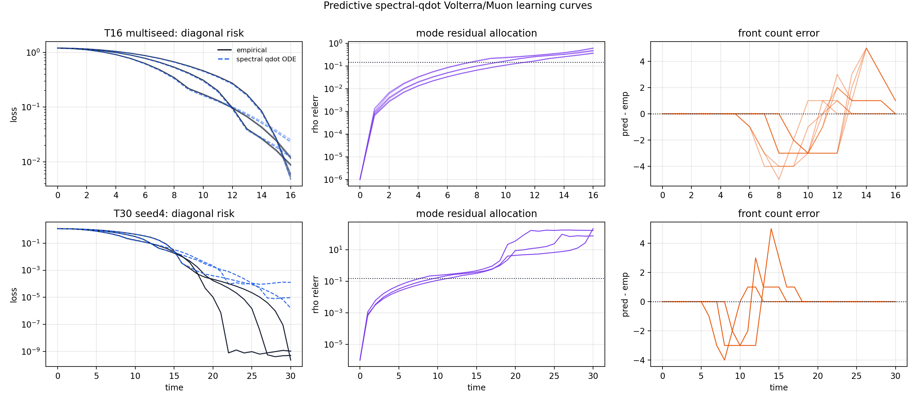
The upper row aggregates the $T=16$ multiseed panel and the lower row shows the longer $T=30$ seed-4 panel. In each row, the left panel compares empirical population risk (solid) with the spectral-$\dot q$ prediction (dashed); the middle panel is the weighted relative $\ell_2$ error between the predicted and empirical residual vectors $\rho(t)$; the right panel is the predicted minus empirical number of modes beyond the half-recovery threshold. The risk and residual-error ordinates are logarithmic. The dotted reference levels are the pre-registered gates $0.15$ for residual error and zero for front-count error.
The quantitative audit is mixed. Over the nine $T=16$ runs, the median log-risk correlation is $0.9989$, median relative risk error is $0.0460$, and median modal-residual error is $0.1007$; six runs pass the preregistered gate and the three $D=40$ runs are held. In the three $T=30$ runs, median log-risk correlation falls to $0.9809$, relative risk error rises to $0.4067$, and all three are held. The maximum front-count error is three to five modes. The figure therefore supports short-horizon shape prediction in part of the panel, not a calibrated long-time learning law.
Status: conditional reduction for the nonlinear stochastic channel; quantitatively tested in finite dimensions.
Layer 3: separating signal from random spectral bulk
The gradient, weights, and Hessian contain a large random component and a finite signal component. The random component creates a dense band of eigenvalues. The signal component can create isolated branches associated with teacher directions.
The exact tool connecting them is a Schur complement: first account for the large random block, then solve a smaller equation for the informative coordinates. A branch is genuinely informative only if it lies outside the bulk and its eigenvector has non-negligible teacher overlap.
For frozen fresh-sample covariance blocks, existing block-Wishart theory gives the limiting bulk and its edges under its assumptions. The finite Schur identities are exact. Their high-dimensional branch predictions additionally require suitable resolvent convergence in the teacher directions.
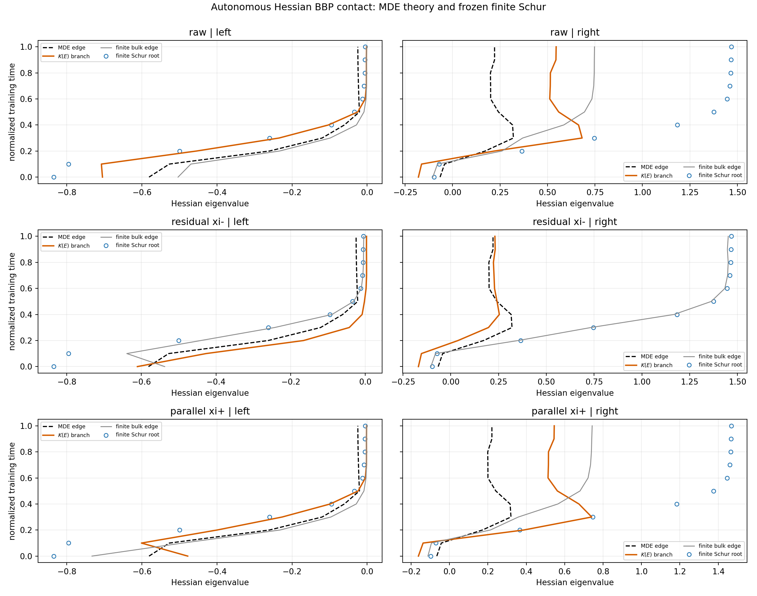
Training time, normalized to $[0,1]$, is vertical and Hessian eigenvalue is horizontal. Rows use three teacher coordinate systems: raw directions, residual directions $\xi^-$, and aligned directions $\xi^+$. Columns show left- and right-edge contacts. The dashed black curve is the deterministic matrix-Dyson edge, the gray curve is the edge of the frozen finite bulk, the orange curve is the deterministic contact branch, and blue circles are roots of the frozen finite-sample Schur kernel.
The run uses $d=24$, width eight, four teacher modes, and 11 training checkpoints. Five of seven deterministic contacts have a stable finite-Schur counterpart; the median and 90th-percentile normalized timing discrepancies are $0.0276$ and $0.0668$. Raw and aligned $\xi^+$ contacts are recovered. The two missing contacts are residual $\xi^-$ branches near the hard edge. Because the blue roots use a finite Schur complement, they are not raw sorted eigenvalue ranks; a separate eigenvector-residue check is required to call a branch teacher-informative.
Status: exact finite decomposition; rigorous frozen bulk under imported assumptions; branch limits conditional on the corresponding directional local law.
Layer 4: controlling the Muon power
Once the reduced state is accepted, the power-selection problem becomes a deterministic control problem with memory. One can differentiate the final objective with respect to the entire power schedule, derive a backward adjoint, and state the correct conditions for an optimal constrained schedule.
These calculations do not depend on an informal analogy with control theory. They are exact for the reduced Volterra model. What remains conditional is the identification of that reduced state with the original same-data stochastic training trajectory.
Status: exact deterministic control calculus for the reduced model; stochastic transfer still conditional.
The central open bridge: reusing the same data
Many random-matrix arguments are cleanest when the matrix being inspected is independent of the parameters. Training does the opposite: the weights are built from the data, and then the gradient or Hessian is computed using those same observations.
This dependence can create bias. It is not legitimate to declare it negligible merely because the dimension is large. A complete theorem needs a uniform leave-one-out comparison: remove one observation, control how much the trajectory changes, and prove that the relevant resolvents remain stable over time and near spectral edges.
This is the main bridge between the fresh-sample theory and the full same-sample training statement.
A separate open problem: critical points at fixed energy
The Hessian along a training trajectory is not the same random object as the Hessian at a critical point selected because its gradient is zero and its loss has a prescribed value.
The second problem belongs to Kac-Rice theory. Conditioning on zero gradient changes the distribution of the Hessian. It therefore needs its own large-deviation and conditioned random-matrix analysis. It should not be presented as a corollary of the Muon trajectory calculation.
The standalone article Energy-Resolved Hessian Spectra in Multi-Index Phase Retrieval explains this distinction. It is related to the spectral program, but it is not a Muon theorem and is not Part II of this series.
How to read the numerical evidence
The experiments test several consequences independently:
- mode-by-mode learning curves;
- bulk spectral density and edge locations;
- informative branch trajectories;
- times at which branches leave the bulk;
- eigenvector overlap with the hidden directions.
Agreement across all of these checks is stronger than matching one final loss value. It still does not replace a proof of the missing uniform same-sample local law.
Takeaway
The project is not one undifferentiated theorem. Its exact core is the finite population reduction, the finite signal-bulk decomposition, and the deterministic control calculus. Established random-matrix results supply frozen fresh-sample bulk laws under explicit assumptions. Experiments support the proposed mode dynamics and spectral crossings. The principal unfinished theorem is the uniform transfer to matrices formed from the same data that generated the trajectory. Energy-conditioned Kac-Rice is a second, distinct frontier.
This separation is the academically useful conclusion: it identifies what can already be used, what is conditional, and precisely what must still be proved.