Muon and controlled training dynamics
Muon for Phase Retrieval I: Learning Hidden Directions with One Fixed Power
Two versions of this work. This page is the accessible version: it explains the problem, the mechanism, and what the experiments mean without assuming knowledge of random matrix theory. The technical paper contains the assumptions, equations, proofs, and numerical protocol.
The problem in one minute
Imagine that a data set hides several useful directions. One direction leaves a strong signal, another leaves a weaker signal, and many others are progressively harder to detect. A learning algorithm does not usually discover all of them at once. It finds the strongest directions first and the weakest ones later.
This post asks a simple question:
Can one fixed setting of the Muon optimizer predict how this sequence of discoveries unfolds?
The model is deliberately simple enough to analyze. It is a version of phase retrieval, where the observations contain squared projections rather than signed linear measurements. Instead of hiding one vector, the teacher hides several orthogonal directions with different strengths. The student must reconstruct the quadratic pattern generated by all of them.
The main conclusion is that training behaves like a moving front. At any time, the strong directions behind the front are already learned, the weak directions ahead of it are still unresolved, and a small group near the front is currently becoming detectable. The Muon power controls how quickly that front moves and how noisy the motion is.
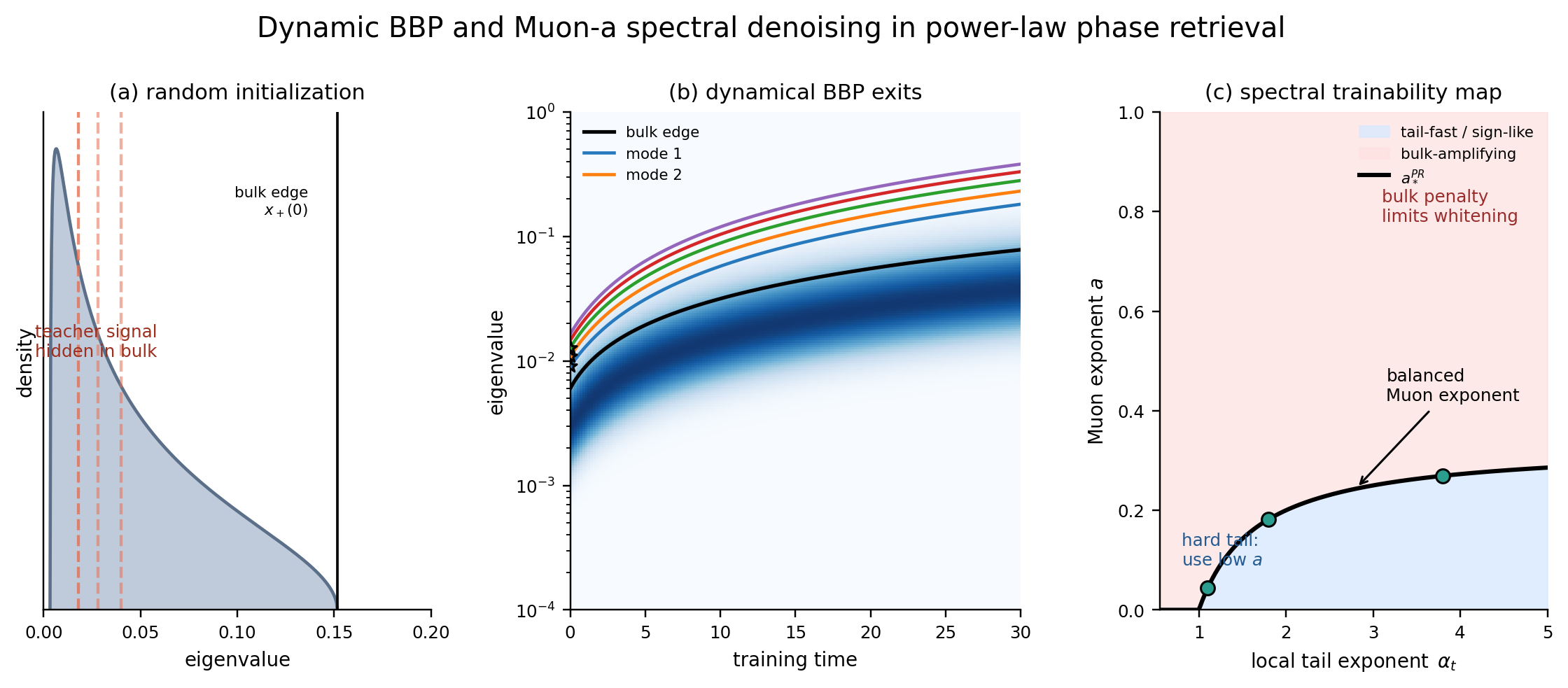
The three panels encode different objects. The left panel is a static signal-plus-bulk cartoon: the solid vertical line is a bulk edge and the dashed teacher locations illustrate hidden and separated signals. The middle panel puts training time on the horizontal axis and eigenvalue on a logarithmic vertical axis; the blue intensity is a moving bulk and the colored curves are teacher-labelled candidate branches. The right panel is a qualitative phase map whose horizontal coordinate is the local tail exponent of the teacher hierarchy and whose vertical coordinate is the Muon power. Its black curve indicates the balance predicted by the reduced asymptotics. None of the three panels reports a confidence interval or an observed transition time.
What phase retrieval means here
In ordinary linear regression, the sign of a projection is observed. In phase retrieval, the sign is lost because the observation depends on its square. A simple one-direction target looks like
\[y=(\theta^\top x)^2.\]The vector $x$ is the input and $\theta$ is the hidden direction. The value of $y$ tells us how strongly $x$ aligns with $\theta$, but it does not tell us on which side of the direction $x$ lies.
The multi-direction version used here adds several such terms. Each hidden direction has a strength. When these strengths decay like a power law, there is no sharp division between “important” and “unimportant” directions: there is a long tail of increasingly weak information.
This model is not intended as a complete description of a large neural network. Its role is to isolate a question that also appears in larger systems: how does an optimizer distribute learning effort across strong and weak spectral directions?
What Muon changes
A matrix gradient has singular values. They measure how strong the update is along different input-output directions. Muon modifies these singular values before applying the update.
If the gradient is decomposed as
\[G=U\,\mathrm{diag}(\sigma_1,\ldots,\sigma_r)V^\top,\]the fixed-power family replaces each $\sigma_j$ by approximately $\sigma_j^a$. The exponent $a$ is the control knob in this post.
- When $a$ is near one, large singular values remain much larger than small ones. The update prioritizes directions that are already strong.
- When $a$ is smaller, the spectrum is flattened. Weak directions receive relatively more attention, but noise near the bottom of the spectrum is amplified as well.
There is therefore no universally best exponent. A useful value must balance two effects: reaching weak teacher directions and avoiding excessive amplification of poorly estimated directions.
Why training has memory
The state of training cannot be described only by the current loss. Two runs can have the same loss while having learned different directions. Their next updates will then behave differently.
The reduced theory keeps track of how much of each hidden direction has been captured. Past updates affect the current gradient, which affects the next update, so the resulting learning-curve equation contains memory. In the technical paper this is written as a Volterra equation. For this blog, the important point is simpler:
The future speed of a direction depends on the entire path that brought training to its current state, not only on the current scalar loss.
Under a fresh-sample approximation, this reduced state predicts the learning curve. The approximation means that the random matrix used to evaluate the next step is treated as independent of the matrices used earlier. Reusing the same training data creates additional dependence; that case is part of the remaining proof program.
Learned is not the same as visible
There are two ways to ask whether a hidden direction has been found.
The first is a population question: does the student align with that direction when averaged over infinitely many fresh inputs? The second is an empirical question: can the direction be identified from a finite matrix computed from the available data?
Finite random matrices contain a dense cloud of noise eigenvalues, called the spectral bulk. A useful direction appears as an isolated eigenvalue only when its signal is strong enough to leave that cloud. This separation is a BBP transition.
An analogy is a solo instrument inside a large orchestra. The melody may already be present, but a listener can identify it only after it becomes loud enough relative to the background. Population alignment says the instrument is playing. Spectral separation says it can be heard on its own.
One training state, three observations
The same hidden learning state can be inspected through three different matrices:
- the gradient, which describes the update proposed now;
- the weights, which contain the accumulated history of past updates;
- the Hessian, which describes the local curvature of the loss.
These matrices do not have the same spectrum, and a direction need not become visible in all three at the same time. The claim is instead that one reduced training state supplies the signal information needed to predict all three observations, once the appropriate random-matrix background is computed for each one.
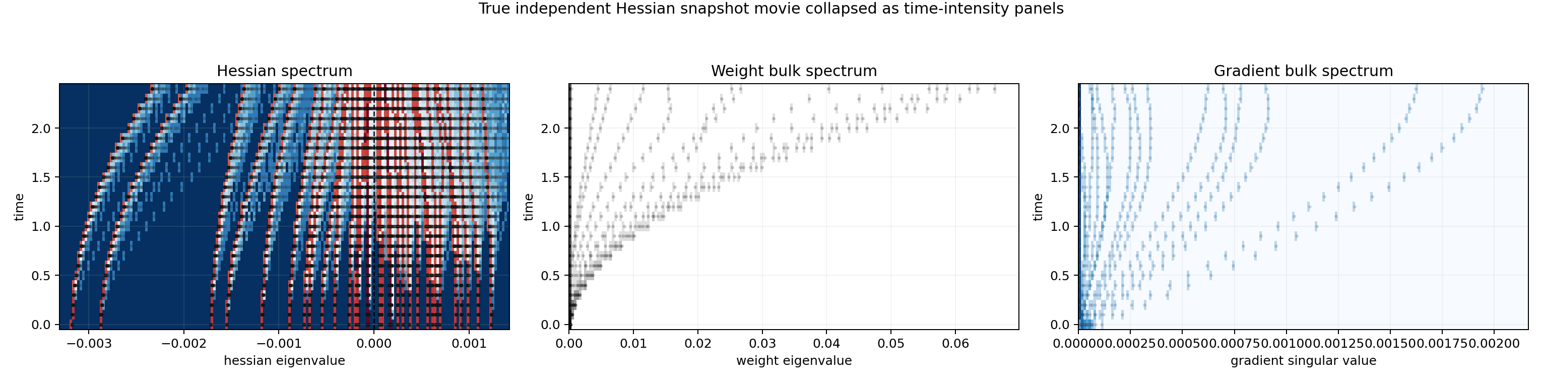
Time runs vertically and the horizontal coordinate is, from left to right, a Hessian eigenvalue, a weight-covariance eigenvalue, and a gradient singular value. Each horizontal slice is an independent fresh spectral snapshot; color intensity is the empirical eigenvalue density accumulated into time bins. The dashed line in the Hessian panel marks zero curvature. The three horizontal scales use different normalizations, so their branch locations must not be compared numerically across panels. The figure shows that the same training state can produce visibly different spectral clocks; it does not identify teacher content because no eigenvector-overlap encoding appears in this raster.
The numerical study checks more than final loss. It compares learning curves, bulk edges, isolated branches, predicted transition times, and the alignment of their eigenvectors with the teacher directions.
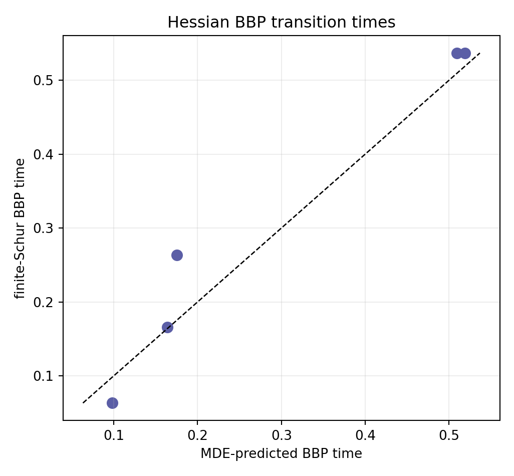
The displayed run has $d=24$, four teacher modes, width eight, and a fresh Hessian aspect ratio of eight. Five of seven deterministic contacts have a stable finite-Schur counterpart. Their median absolute discrepancy is $0.0276$ and their 90th-percentile discrepancy is $0.0668$ after normalizing training time to $[0,1]$. The two unmatched predictions are residual $\xi^-$ contacts near the hard edge; they are not assigned to whichever sorted eigenvalue happens to be closest. This is a comparison of a deterministic contact calculation with a frozen finite-sample Schur calculation, not a same-data training theorem.
Mathematical scope
The finite-dimensional population algebra is exact: the quadratic Gaussian model closes on the student–teacher Gram state, and the singular-value transformation defining the fixed-power update is an exact matrix operation.
The Volterra memory equation is exact for the reduced modal equation, but its identification with nonlinear empirical training uses the stated fresh projected-gradient channel hypothesis. For a fixed finite Hessian, the Schur complement and its residue are algebraic identities. Replacing the finite bulk resolvent by a deterministic one uses a bounded fresh-sample random-matrix limit and directional resolvent control.
The plots test individual links in that chain. They do not prove a time-uniform local law for a trajectory trained and evaluated on the same finite observations, and the unmatched hard-edge contacts show where the finite diagnostic is not yet complete.
Takeaway
The original problem was to understand how one fixed Muon power learns a hierarchy of hidden directions. The answer is not simply “smaller is better” or “larger is better.” The exponent moves a spectral front while trading weak-signal resolution against noise amplification. A reduced state predicts the learning curve, and random-matrix tests determine when each learned direction becomes visible in the gradient, weights, or Hessian.
The next Muon article asks what happens when the exponent is allowed to change during training: Choosing the Muon Power During Training.