Spectral transitions in multi-index models
When the Output Weights Learn: Joint Dynamic BBP Transitions
This article is the output-feature companion in the phase-retrieval research program. It uses the same spectral language while keeping the trainable output amplitudes distinct from the Muon spectral power.
In the usual quadratic multi-index model, the second-layer coefficients are often fixed:
\[f_W(x)=\frac1p\sum_{r=1}^p(w_r^\top x)^2.\]That choice hides a second learning problem. If the coefficients are trained,
\[f_{a,W}(x)=\frac1p\sum_{r=1}^p a_r(w_r^\top x)^2,\]then the network must learn both a subspace and a distribution of amplitudes inside that subspace. These two tasks interact, but they are not the same.
This article isolates that interaction. It is a companion to the energy-resolved Kac–Rice analysis, not a statement about Muon. The exact results are the joint population equations, the full Hessian blocks, the rank criterion, and the finite Schur reduction. For a bounded smooth link, the orthogonal weight bulk also falls exactly under the block-Wishart theorem, which supplies its density, support edges, and logarithmic potential. The pure quadratic tail extension and the limiting coupled BBP theorem still require additional estimates, while the proposed effective-width criterion remains a conjecture.
The risk forgets the decomposition
Write
\[A=\operatorname{diag}(a_1,\ldots,a_p), \qquad B=\frac1pWAW^\top, \qquad A_\star=\Theta\Lambda\Theta^\top.\]The Gaussian population risk depends only on $E=B-A_\star$:
\[R(a,W) = \operatorname{Tr}(E^2) +\frac12\bigl(\operatorname{Tr}E\bigr)^2.\]This creates a useful tension. The risk sees the learned matrix $B$, but the parameterization contains its individual atoms $(a_r,w_r)$. For any invertible diagonal matrix $D$,
\[W\longmapsto WD, \qquad A\longmapsto D^{-2}A\]leaves $B$ unchanged. The Euclidean gradient flow is not invariant under this rescaling. Two networks representing exactly the same function can therefore have different future trajectories and different spectral transition times.
The exact joint dynamics
Set
\[L=2E+\operatorname{Tr}(E)I_d, \qquad Q=W^\top W, \qquad M=W^\top\Theta.\]The population gradients are
\[\nabla_WR=\frac2pLWA, \qquad \nabla_aR=\frac1p\operatorname{diag}(W^\top LW).\]Define
\[S=\frac2pQAQ-2M\Lambda M^\top+\tau Q,\] \[T=\frac2pQAM-2M\Lambda+\tau M, \qquad \tau=\frac1p\operatorname{Tr}(AQ)-\operatorname{Tr}\Lambda.\]Then the entire population flow closes on the finite state $(a,Q,M)$:
\[\dot Q=-\frac2p(AS+SA), \qquad \dot M=-\frac2pAT, \qquad \dot a=-\frac1p\operatorname{diag}S.\]For frozen unit coefficients, the captured teacher matrix
\[C=M^\top Q^{-1}M\]satisfies an autonomous Riccati equation. That autonomy disappears when $a$ is trained: the factors of $A$ do not cancel. Subspace capture is no longer a complete state description.
What must be measured in the output layer
The teacher-sector quadratic form is
\[K_\Theta=\frac1pM^\top AM.\]$C$ says whether the student span contains a teacher direction. $K_\Theta$ says whether the learned quadratic form has the right amplitude in that direction. The residual state therefore contains both
\[I_k-C \qquad\text{and}\qquad \Lambda-K_\Theta.\]The distribution of output mass can be summarized by
\[N_{\mathrm{eff}}^+(a) = \frac{\left(\sum_r(a_r)_+\right)^2} {\sum_r(a_r)_+^2}.\]This participation number equals $p$ for balanced positive coefficients and approaches one when almost all positive mass is concentrated on one atom. It is not a sufficient statistic for the dynamics, but it immediately detects nominal width that is not being used.
The Hessian has three kinds of branches
For one observation, let
\[h=W^\top x, \qquad y=\Theta^\top x, \qquad s=\frac1p\sum_r a_rh_r^2-y^\top\Lambda y.\]The weight–weight Hessian is a weighted covariance matrix. Its student-index weight is
\[A^{WW}(a,h,y) = \frac4{p^2}(Ah)(Ah)^\top+\frac{2s}{p}A.\]This block carries the high-dimensional random-matrix bulk. The output–output block has only dimension $p$,
\[H^{aa}_{rs} = \frac1{np^2}\sum_{\ell=1}^n h_{\ell r}^2h_{\ell s}^2,\]and a mixed block couples it to the weights. The output coordinates do not change the limiting bulk density when $p$ is fixed, but they do change every finite outlier equation.
The weight bulk is exactly block-Wishart
For a smooth feature link $\varphi$, write
\[r_i=\frac1p\sum_r a_r\varphi(h_{ir}) -\sum_j\mu_j\varphi(y_{ij}), \qquad g_i=\frac1p a\odot\varphi'(h_i),\]and define the $p\times p$ Hessian weight
\[T_i=g_ig_i^\top +r_i\operatorname{diag}\!\left( \frac1p a\odot\varphi''(h_i) \right).\]Let $U$ span the orthogonal complement of $\operatorname{span}(W,\Theta)$ and put $\xi_i=U^\top x_i$. Gaussian orthogonality makes $\xi_i$ independent of $(h_i,y_i)$. Conditionally on the finite projections, the orthogonal weight Hessian is exactly
\[H_\perp^{WW} =\frac1n\sum_{i=1}^n (I_p\otimes\xi_i)T_i(I_p\otimes\xi_i^\top).\]This is the indefinite block-Wishart ensemble studied by Montanari and Saeed. If the law $\nu$ of $T_i$ is compactly supported and $n/d_0\to\alpha$, define
\[\mathscr K_{\alpha,\nu}(S) =\int T(I_p+ST)^{-1}\,\nu(dT)-\frac1\alpha S^{-1}.\]The matrix Stieltjes transform solves
\[\mathscr K_{\alpha,\nu}(S(z))=zI_p, \qquad m(z)=\frac\alpha p\operatorname{Tr}S(z).\]For
\[\mathcal P_- =\left\{S\succ0: S^{-1}+T\succ0\ \text{on }\operatorname{supp}\nu, \ D\mathscr K(S)\succ0\right\},\]the left edge is
\[\zeta_- =\sup_{S\in\mathcal P_-} \lambda_{\min}\!\left(\mathscr K_{\alpha,\nu}(S)\right).\]The right edge follows by reflecting every block, $T\mapsto-T$. For $u<\zeta_-$, the normalized logarithmic potential is
\[\int\log|\lambda-u|\,\mu_{\alpha,\nu}(d\lambda) =\frac1p\inf_{S\in\mathcal P_-} \left[ -\alpha u\operatorname{Tr}S +\alpha\int\log\det(I_p+TS)\,\nu(dT) -\log|\det S|-p(\log\alpha+1) \right].\]For the pure quadratic link $\varphi(u)=u^2$, the Gaussian block weights are unbounded. The theorem-ready comparison uses
\[\varphi_L(u)=L^2\tanh(u^2/L^2),\]whose value and first two derivatives are bounded. Returning to the pure quadratic model requires a separate growing truncation and a uniform tail-and-stability proof.
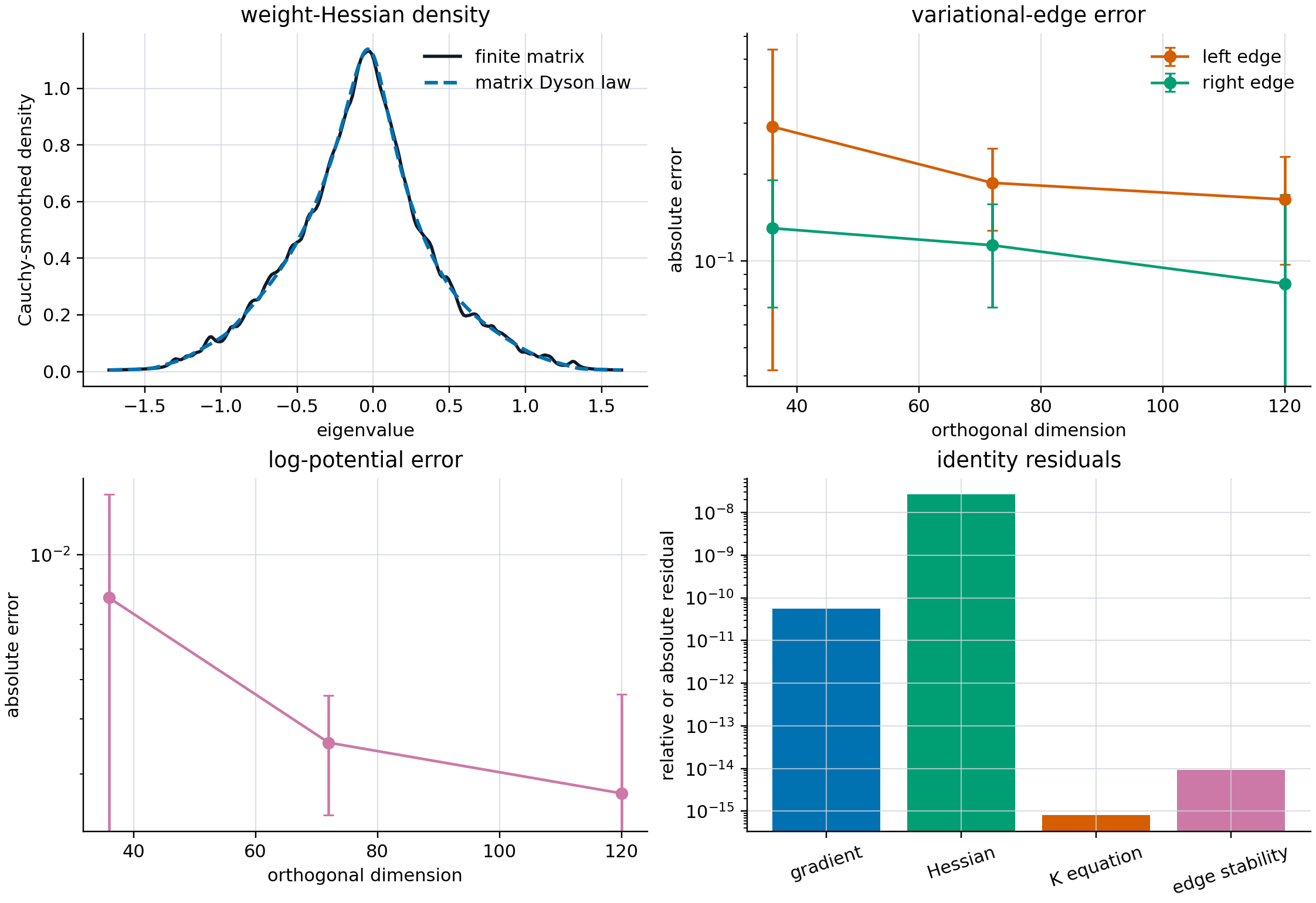
At the largest tested dimension, the smoothed-density relative $L^1$ error is $0.0297$. The mean absolute errors are $0.1634$ for the left edge, $0.0834$ for the right edge, and $0.00174$ for the logarithmic potential. The analytic gradient and Hessian directional errors are respectively $5.67\times10^{-11}$ and $2.66\times10^{-8}$.
The right finite sector is
\[\mathcal F = \bigl(\operatorname{span}(W,\Theta)\otimes\mathbb R^p\bigr) \oplus\mathbb R_a^p.\]The student span must be included because it can carry finite but non-informative rotation or amplitude directions. After integrating out the remaining orthogonal weight bulk, one obtains a finite Schur matrix $K(z)$. All isolated branches solve one equation:
\[\det\bigl(K(z)-zI_{\mathcal F}\bigr)=0.\]If the finite kernel vector is $c=(c_W,c_a)$, the derivative of the same matrix gives the residues
\[\Omega_a = \frac{\lVert c_a\rVert^2} {c^\top\bigl(I-\partial_zK(z)\bigr)c}, \qquad \Omega_\Theta = \frac{\lVert\Pi_\Theta c_W\rVert^2} {c^\top\bigl(I-\partial_zK(z)\bigr)c}.\]Here $\Pi_\Theta$ projects the finite weight sector onto the teacher directions. Student-internal finite directions may create isolated eigenvalues, but they are not informative about the teacher.
This gives a precise attribution:
- an output branch has non-vanishing $\Omega_a$ and vanishing $\Omega_\Theta$;
- a teacher-weight branch has non-vanishing $\Omega_\Theta$ and vanishing $\Omega_a$;
- a mixed branch has both.
The classification follows the branch through crossings. Sorting empirical eigenvalues by rank cannot do that reliably.
What does (p>k) really mean?
There is one exact statement:
A rank-$k$ positive teacher can be represented exactly if and only if $p\geq k$.
Necessity is rank counting. Sufficiency follows by taking $w_i=\sqrt{p\mu_i}\theta_i$ and $a_i=1$ for the first $k$ atoms.
Nothing in this proof says that $p>k$ automatically separates output and weight BBP events. A wide network can still concentrate its useful mass on only $k$ atoms. Conversely, one redundant, well-balanced atom may already create a genuine finite-sector slack.
For an active teacher group $J$, define the atom contribution
\[b_r(J)=(a_r)_+ \left\lVert P_J\Theta^\top w_r\right\rVert^2\]and its sector participation
\[N_{\mathrm{eff},J}^+ = \frac{\left(\sum_rb_r(J)\right)^2}{\sum_rb_r(J)^2}.\]The conjectured regularity condition is
\[N_{\mathrm{eff},J}^+>|J|.\]It says that the active teacher front should be supported by more effective atoms than active modes. This is a plausible condition for separating amplitude and subspace events, but it is not yet a theorem: the finite Schur kernel also needs transversality and non-degenerate residues.
What the finite experiment shows
The diagnostic integrates the exact population flow, then builds the full Hessian from an independent Gaussian sample. It uses $k=3$, dimensions $d=28$, aspect ratio $n/d=6$, widths $p=3,4,6$, and three seeds. The initial outputs are lognormal and normalized to mean one.
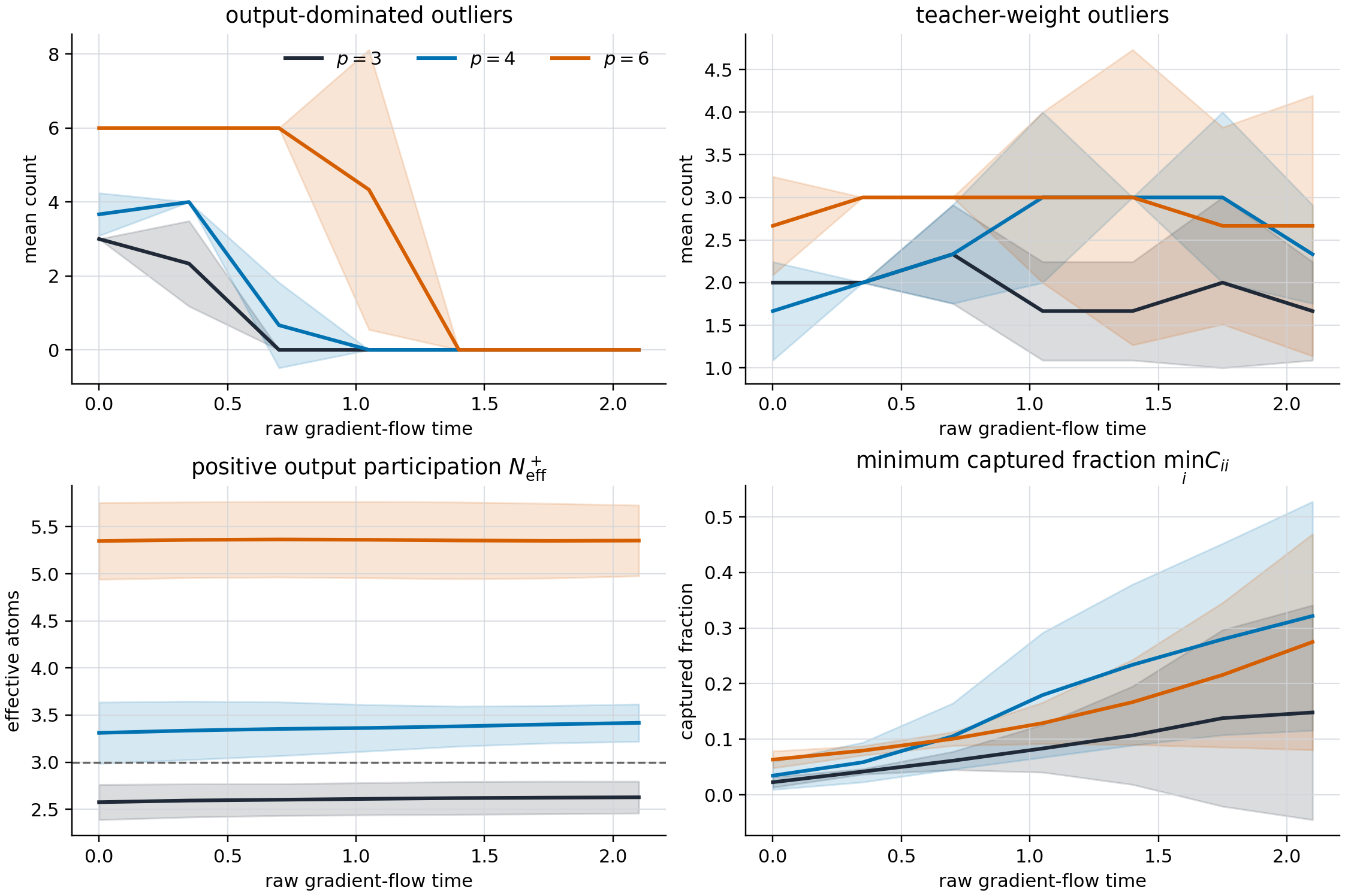
At initialization, the mean counts of output-dominated outliers are $3.0$, $3.67$, and $6.0$ for $p=3,4,6$. By the final snapshot they have all returned to the empirical weight-bulk interval, while teacher-weight branches remain. The final positive participation rises with $p$, but the minimum captured teacher fraction is not monotone at the same raw time.
The experiment therefore supports a limited conclusion: width alone is not the control variable. It does not prove the effective-slack conjecture. A decisive test needs matched clocks, dimension scaling, more seeds, and the deterministic joint Schur roots rather than empirical bulk quantiles.
The remaining theorem
The main missing probabilistic input is a uniform anisotropic local law for the mixed output–weight vectors inside the weighted covariance resolvent. It must control both the Schur kernel and its spectral derivative; locations alone are insufficient because branch attribution comes from residues.
Four further extensions remain separate:
- a uniform truncation-removal theorem for the pure quadratic block weights;
- a leave-one-out comparison when the training and Hessian samples coincide;
- a non-degeneracy theorem connecting sector participation to separated roots;
- for the energy-conditioned problem, the continuum Kac–Rice saddle and the local law after conditioning the full gradient to vanish.
The exact algebra has reduced the question to a finite kernel. The hard part is now sharply located: prove that this kernel is the deterministic limit of the empirical coupled Hessian along the trajectory.