General-Link Gaussian Multi-Index Models: Gradient, Weight, and Hessian Spectra

Quadratic phase retrieval is often the first model where the algebra becomes transparent. If

\[f_W(x)=\frac1p\sum_{a=1}^p(w_a^\top x)^2, \qquad f_\star(x)=\sum_{i=1}^k\mu_i(\theta_i^\top x)^2,\]

then the population dynamics closes on a few overlaps:

\[Q=W^\top W, \qquad M=W^\top\Theta.\]

It is natural to ask whether this closure is a quadratic miracle. It is not. The real reason is Gaussianity. A Gaussian vector only remembers a finite set of projections through their covariance matrix.

This post explains the general-link version:

\[f_W(x)=\sigma(W^\top x), \qquad f_\star(x)=g(\Theta^\top x),\]

where (\sigma:\mathbb R^p\to\mathbb R) and (g:\mathbb R^k\to\mathbb R) may be non-polynomial smooth functions.

The conclusion has several levels. The population reduction below is exact for links with sufficient Gaussian integrability. Existing effective spectral theory rigorously covers each diagonal Hessian block under its hypotheses. The complete block Hessian requires a matrix-weighted extension, and polynomial links additionally require uniform removal of truncation.

The population reduction

Let

\[h=W^\top x,\qquad y=\Theta^\top x, \qquad \Delta(h,y)=\sigma(h)-g(y).\]

For the square loss

\[R(W)=\frac12\mathbb E\Delta(W^\top x,\Theta^\top x)^2,\]

define the joint Gram matrix

\[G= \begin{pmatrix} Q&M\\ M^\top&I_k \end{pmatrix}.\]

If (U=(h,y)\sim N(0,G)) and

\[\Psi(h,y)=\Delta(h,y)\nabla\sigma(h), \qquad \Xi(G)=\mathbb E_G[U\Psi(U)^\top],\]

then

\[\Gamma(G)=G^\dagger\Xi(G) = \begin{pmatrix} \Gamma_h\\ \Gamma_y \end{pmatrix}\]

gives the exact population gradient

\[\nabla_W R(W)=W\Gamma_h+\Theta\Gamma_y.\]

Therefore the flow closes on the finite summaries:

\[\dot Q =-\Gamma_h^\top Q-Q\Gamma_h-\Gamma_y^\top M^\top-M\Gamma_y,\] \[\dot M =-\Gamma_h^\top M-\Gamma_y^\top.\]

No ambient-dimensional state remains. The input dimension enters only through initialization and finite-sample fluctuations.

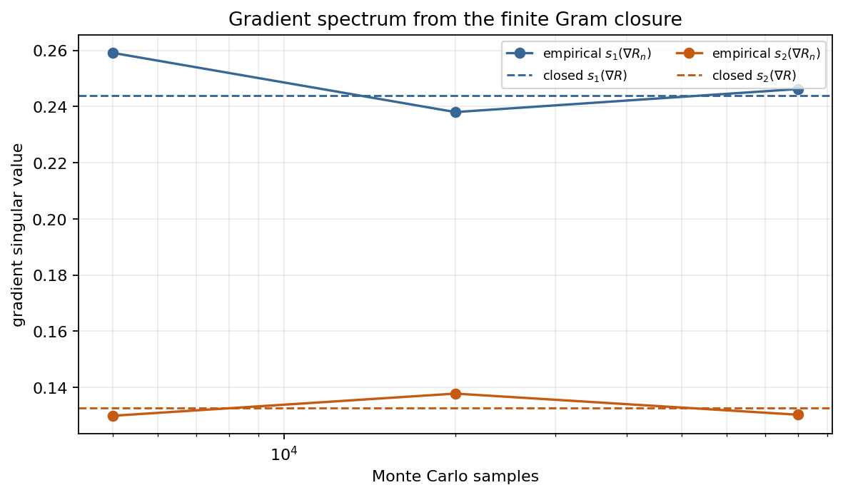
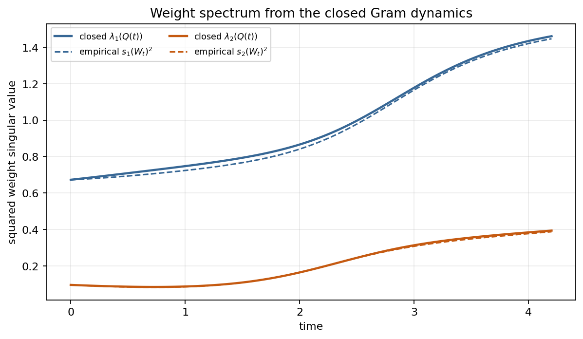
The same closure gives two spectral identities. The squared singular values of the population gradient are the eigenvalues of

\[\mathcal G_\nabla(Q,M)=\Gamma(G)^\top G\Gamma(G),\]

while the squared singular values of the weights are simply the eigenvalues of (Q). For a simple eigenpair ((q_i,v_i)),

\[\dot q_i=-2q_i v_i^\top\Gamma_hv_i-2v_i^\top M\Gamma_yv_i.\]

Thus gradient and weight spectra are exact finite-Gram observables, not additional high-dimensional order parameters.

Why Hermite coordinates are natural

For Gaussian data, the Hermite basis is the diagonal language of the model. Write, formally,

\[\sigma(h)=\sum_\alpha a_\alpha \widehat{\mathrm{He}}_\alpha(h), \qquad g(y)=\sum_\beta b_\beta \widehat{\mathrm{He}}_\beta(y).\]

For finite Hermite expansions, the entries of (\Xi(G)) are finite Wick contractions. This is the Hermite-DMFT form of the population dynamics: a low-dimensional Gaussian covariance evolves deterministically, and Hermite coefficients decide which directions can escape a saddle.

In the diagonal single-index picture, if the first nonzero Hermite coefficient has degree (s) and initialization has overlap (m(0)\asymp d^{-1/2}), the escape scales are

\[T_s(d)\asymp \begin{cases} 1,&s=1,\\ \log d,&s=2,\\ d^{(s-2)/2},&s>2. \end{cases}\]

This is the same information-exponent mechanism emphasized in work on Gaussian multi-index models by Bietti, Bruna, and Pillaud-Vivien, and in the phase-retrieval dynamics of Braun, Loureiro, Quang Minh, and Imaizumi.

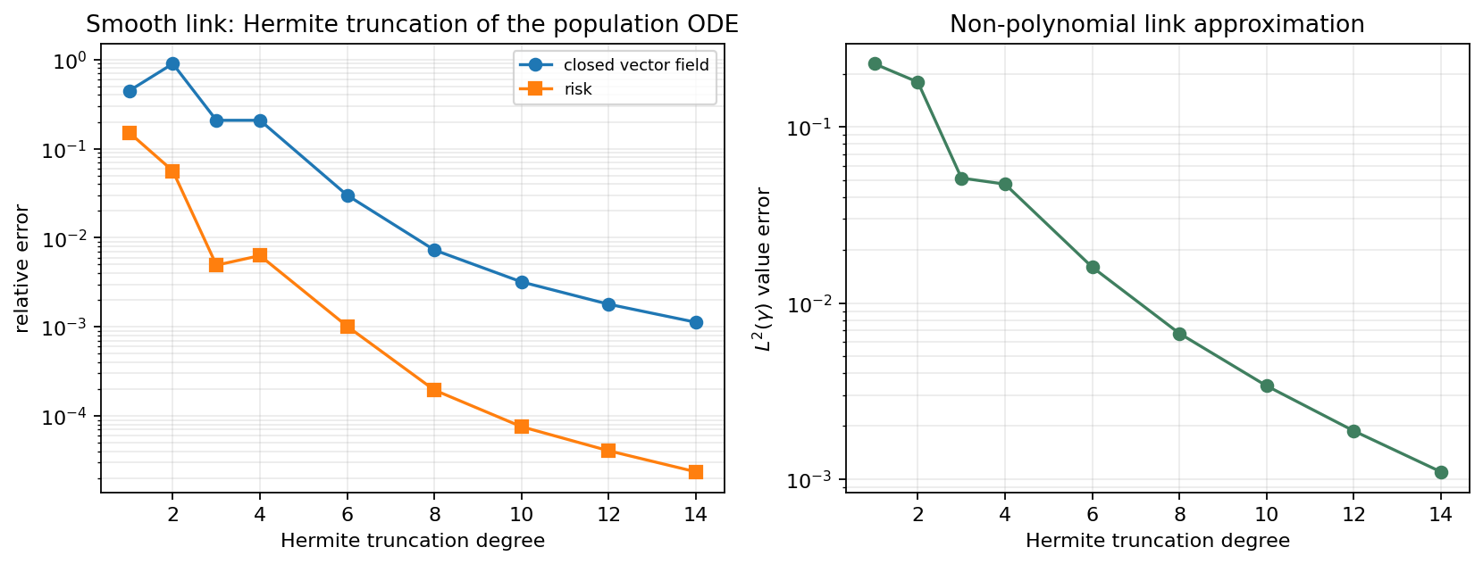
Finite Hermite polynomials are not a limitation. For a smooth non-polynomial link, project onto degree (L) and let (L\to\infty). On any compact, non-degenerate set of Gram matrices, convergence in the relevant Gaussian Sobolev norms gives uniform convergence of the vector field. Gronwall’s inequality then gives convergence of the projected trajectories on every finite time interval on which they remain in that set.

The empirical Hessian is still a weighted covariance matrix

Now fix (W) and draw an independent sample (x_1,\ldots,x_n). The Hessian with respect to the columns of (W) has blocks

\[H_{ab}(W)=\frac1nX^\top D_{ab}(W)X.\]

The diagonal weights are

\[D_{ab,\ell}(W) =A_{ab}(W^\top x_\ell,\Theta^\top x_\ell),\]

where

\[A(h,y) = \nabla\sigma(h)\nabla\sigma(h)^\top +\Delta(h,y)\nabla_h^2\sigma(h).\]

This identity is finite-dimensional and exact. Random-matrix theory enters only after this algebraic reduction. For a fixed (a), the diagonal block (H_{aa}) has scalar weight (A_{aa}(h,y)) and is covered by the effective spectral framework of Ben Arous, Gheissari, Huang, and Jagannath under its support and non-degeneracy assumptions. Their theorem gives its scalar bulk law and a finite outlier determinant.

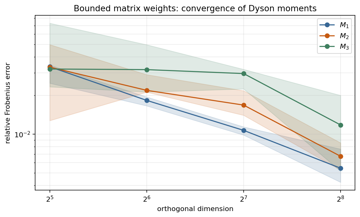
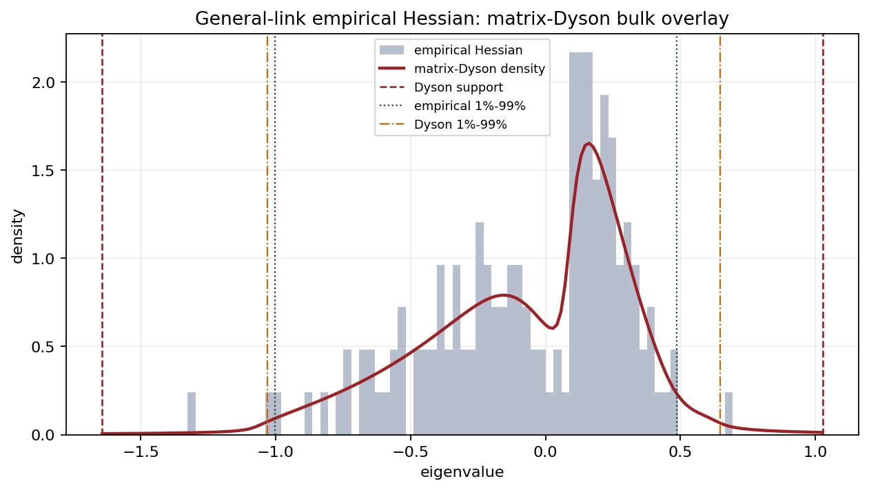
The complete (pd\times pd) Hessian is a different random matrix: its sample weights are the matrices (A(h,y)), and every block shares the same covariate. For bounded matrix weights, its global spectral law can nevertheless be proved directly. The proof expands normalized matrix moments, keeps the noncrossing Wick contractions, and sums their noncommutative recursion. If (S(z)) is the limiting matrix Stieltjes transform, the result is

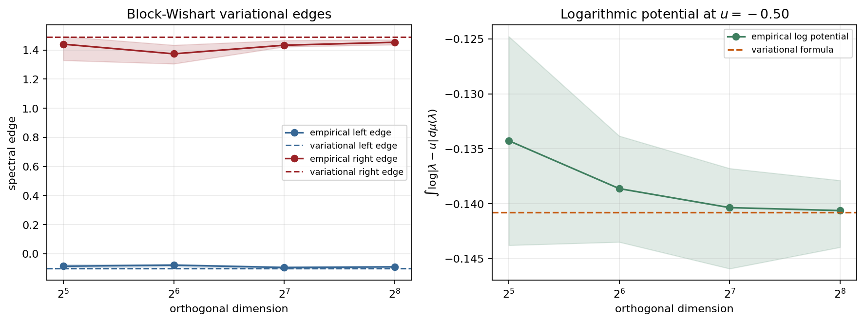
\[-S(z)^{-1} =zI_p- \mathbb E\left[A\left(I_p+\alpha^{-1}S(z)A\right)^{-1}\right].\]

Thus the matrix-Dyson equation is a theorem for the global bulk under bounded weights. Montanari and Saeed’s block-Wishart variational theorem strengthens this statement: it gives both support edges and the logarithmic potential outside the support. With

\[\mathbb K_{\alpha,\nu}(U) =\mathbb E_\nu[A(I+UA)^{-1}]-\alpha^{-1}U^{-1},\]

the left edge is

\[\zeta_-=\sup_{U\in\mathcal P_-} \lambda_{\min}(\mathbb K_{\alpha,\nu}(U)),\]

where (\mathcal P_-) imposes positivity before the poles and positivity of the derivative (D\mathbb K). The right edge follows by replacing (A) with (-A). For (u<\zeta_-), the same paper gives a variational formula for (\int\log|\lambda-u|\,d\mu(\lambda)). In particular, it supplies the bulk Kac–Rice log determinant at (u=0) whenever the lower edge is strictly positive. It does not cover the singular case where zero lies inside the bulk.

There is an exact reduction behind that open problem. Let (B=[W,\Theta]) and split a Gaussian covariate into

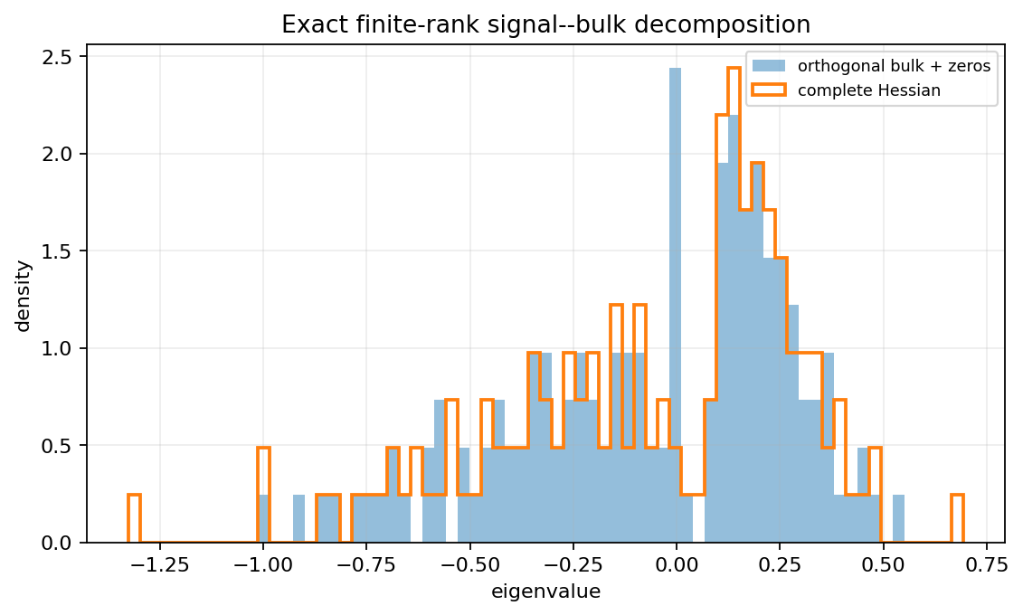
\[x=Lz+L_\perp\xi, \qquad L=BG^{-1/2}.\]

The weight (A) depends only on (z), while (\xi) is an independent standard Gaussian in dimension (d-p-k). After this change of basis, the full Hessian differs by rank at most (2p(p+k)) from

\[B_n=\frac1n\sum_{\ell=1}^n A(G^{1/2}z_\ell)\otimes\xi_\ell\xi_\ell^\top.\]

Thus the finite signal sector cannot change the limiting bulk. The remaining task is sharply localized: obtain anisotropic resolvent control, then put the finite signal sector back by a Schur complement. The scalar bulk edges themselves are no longer part of this open task.

BBP roots and teacher visibility

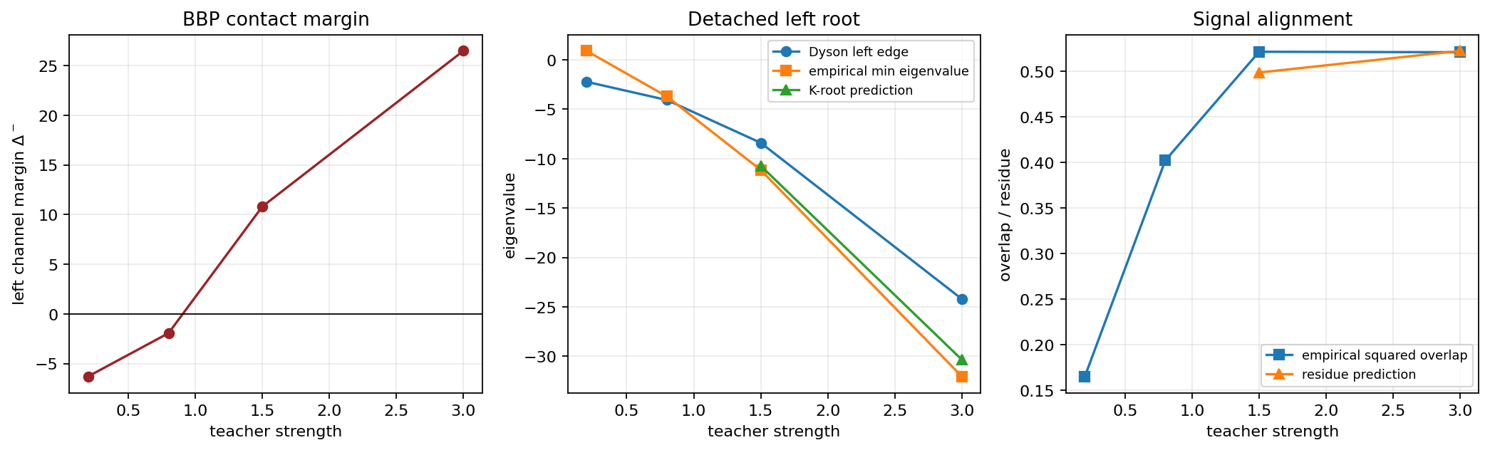
Let (S(z)) be the matrix Stieltjes solution outside the bulk. For the complete Hessian, the still-conjectural Schur-channel diagnostic associated with a normalized teacher projection (\zeta) is

\[K_\zeta(z) = \mathbb E\left[ \zeta^2 A(h,y) \left(I_p+\alpha^{-1}S(z)A(h,y)\right)^{-1} \right], \qquad \alpha=\frac nd.\]

A simple left outlier branch is a solution of

\[\lambda_{\rm out} =\lambda_{\min}K_\zeta(\lambda_{\rm out}), \qquad \lambda_{\rm out}<x_-.\]

A right branch uses the maximal eigenvalue and the right edge (x_+). With the scalar channel normalization above, the same branch gives the squared-overlap diagnostic

\[\Omega_{\rm out} = \frac1{1-\partial_z k(\lambda_{\rm out})}.\]

This distinction is important: population learning and empirical spectral visibility are different events. A teacher direction can be represented in the population state before the empirical Hessian has an isolated eigenvector that points toward it.

What is exact, and what is asymptotic?

There are six logical layers.

1. Exact population algebra.
   The closure on ((Q,M)) follows directly from Gaussian conditioning.

2. Exact finite Hessian algebra.
   The block formula (H_{ab}=n^{-1}X^\top D_{ab}X) holds before taking any limit, as does the finite-rank signal–bulk decomposition.

3. Asymptotic theory for diagonal blocks.
   For bounded scalar weights satisfying the support and non-concentration assumptions, each (H_{aa}) has the rigorous bulk and finite-channel theory proved by Ben Arous et al.

4. Bulk theory for the complete Hessian.
   For uniformly bounded matrix weights, the noncrossing moment expansion proves convergence of the full bulk and the matrix-Dyson equation; Montanari–Saeed gives its support edges and exterior logarithmic potential.

5. Complete-Hessian outlier prediction.
   The Schur-channel equations require an anisotropic local law beyond both the global moment theorem and the cited scalar-block theorem.

6. Polynomial-link extension.
   The plotted cubic-Hermite BBP roots use unbounded Hessian weights. They are experimentally stable predictions, but a journal-level theorem still needs estimates uniform in the truncation threshold, including control at the bulk edge and of the derivative entering the overlap residue.

This separation keeps the story honest. The Hermite-DMFT reduction is not a numerical ansatz: it is an exact finite-dimensional population identity. The scalar diagonal-block random-matrix step is an existing theorem, and the bounded full-Hessian bulk, support edges, and exterior log potential are now rigorous. The next theorem is anisotropic: the full Schur determinant, its outliers, and the corresponding eigenvector projections.

Further reading

• A. Bietti, J. Bruna, and L. Pillaud-Vivien, On Learning Gaussian Multi-index Models with Gradient Flow.
• G. Braun, B. Loureiro, H. Quang Minh, and M. Imaizumi, Fast Escape, Slow Convergence: Learning Dynamics of Phase Retrieval under Power-Law Data.
• G. Ben Arous, R. Gheissari, J. Huang, and A. Jagannath, Local geometry of high-dimensional mixture models.
• A. Montanari and B. Saeed, Variational Formulas for the Spectrum of Block Wishart Matrices.

The companion manuscript contains the precise assumptions, proofs, experimental protocol, and open theorem boundary.