This series asks a concrete question: can a transformer use a short prompt of PDE examples to solve a new PDE query from the same task?
This first post removes the hardest part. The PDE operator is fixed. A numerical Galerkin method has already turned the PDE into one linear system, and the transformer is only tested as a fast reusable decoder for many new right-hand sides. In numerical-analysis language, the decoder should behave like a learned preconditioner.
The figures below are diagnostic simulations. They are meant to make the solver mechanism readable before the later posts add unknown PDE coefficients, statistical task variation, and replica-theory questions.
The cleanest case is the one where the PDE coefficient is not task-dependent. Take a linear elliptic equation on a bounded domain,
\[-\nabla\cdot(a\nabla u)+Vu=f,\qquad u|_{\partial\Omega}=0,\]and suppose for this first note that (a) and (V) are fixed across tasks. After Galerkin discretization, every prompt pair ((f_i,u_i)) satisfies the same finite-dimensional system
\[A u_i=f_i .\]The in-context problem is therefore not to infer a new operator. The operator is fixed. The problem is to learn how to apply (A^{-1}) quickly to a new query source (f_\star).
That makes the decoder the central object. A depth-(L) decoder can be viewed as a recurrent solver
\[u_{\ell+1}=u_\ell+P_\theta(f_\star-Au_\ell),\]where (P_\theta) is the preconditioner represented by the trained attention and feed-forward layers. The exact error identity is
\[e_L=(I-P_\theta A)^L e_0,\qquad e_\ell=u_\ell-u_\star.\]So the role of depth is transparent: each layer is one solver step. The generalization question is not whether the model memorized a particular source, but whether the learned preconditioner works on new right-hand sides drawn from the same source distribution.
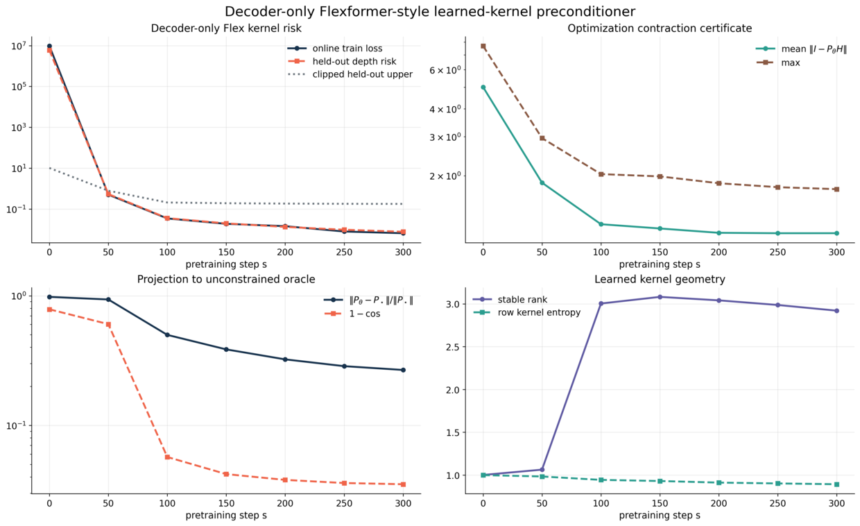
Compact diagnostic plots (simple experiments)
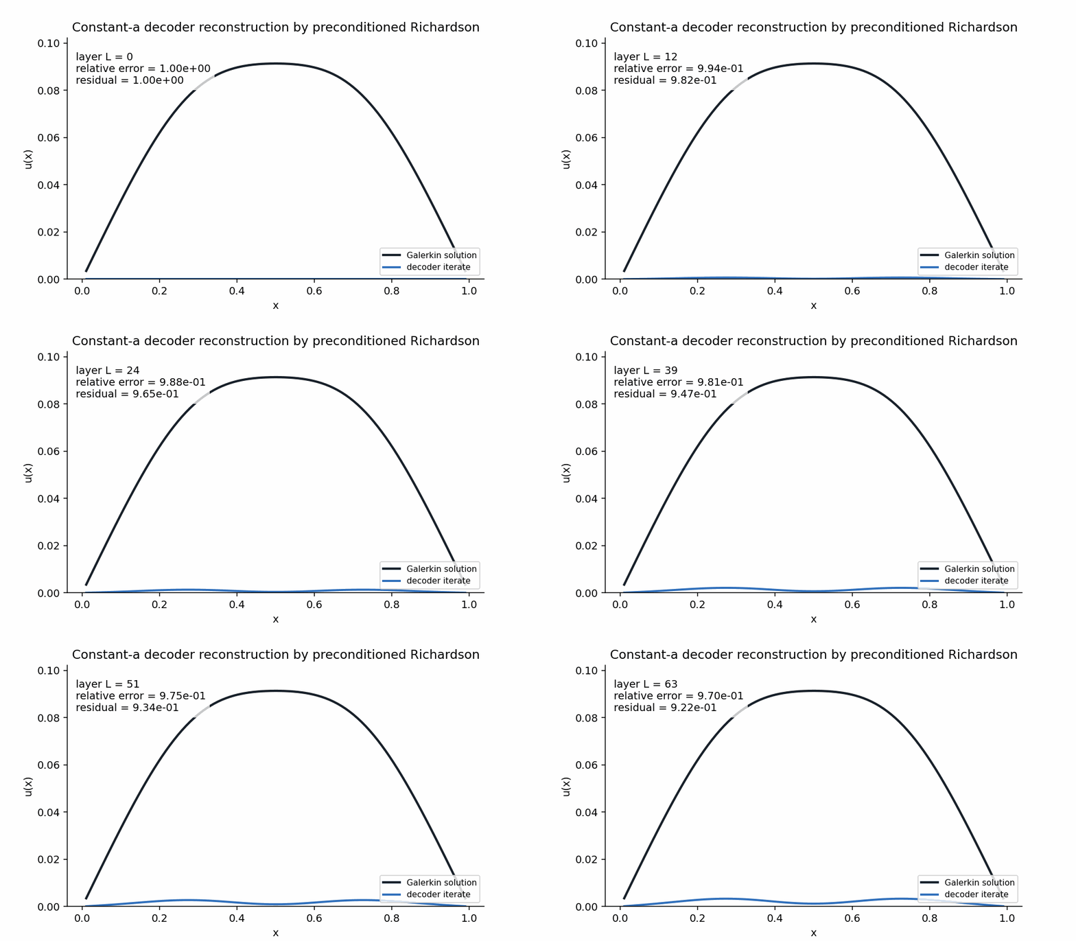 The animation shows the decoder as an iterative solver. The black curve is the Galerkin solution \(u_\star=A^{-1}f_\star\). The blue curve is the depth-\(L\) decoder iterate. In the constant-\(a\) case, this is the cleanest possible visual test: the model is not changing the operator, it is only improving the reconstruction of the solution for a fixed linear system. 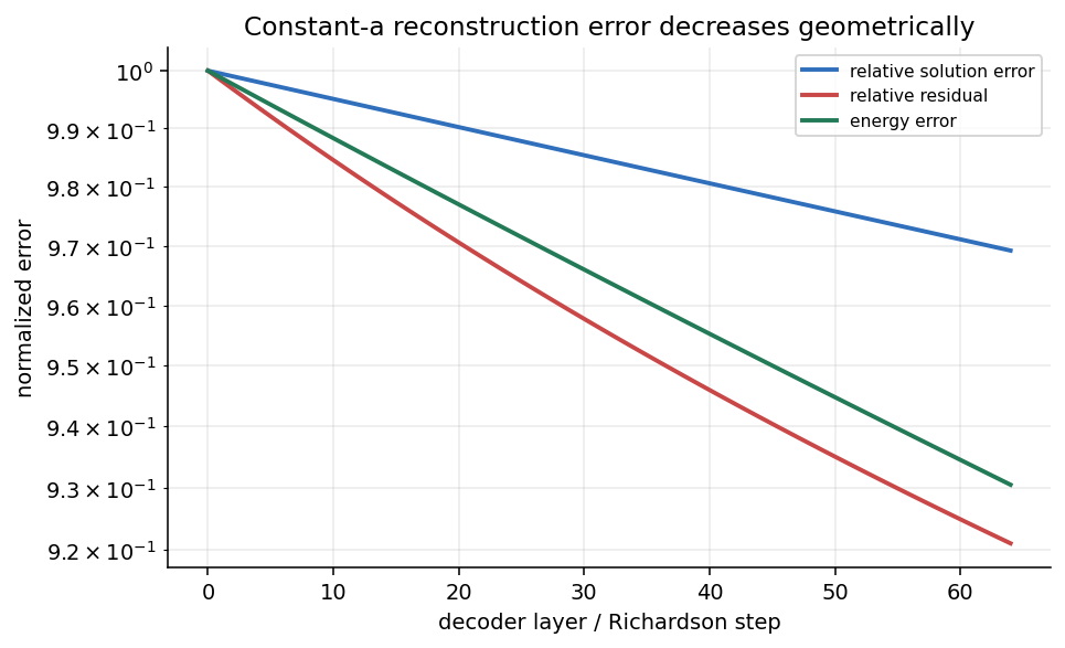 The residual, solution error, and energy error all fall together. This is what one expects if the decoder has really learned a preconditioned Richardson step rather than only fitting the pointwise solution curve. Residual decay means the iterate is satisfying the Galerkin equation; energy decay means it is improving in the PDE norm. 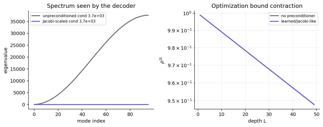 The spectrum plot is the preconditioner story in one picture. Without preconditioning, the wide spectrum forces a slow worst-mode contraction. A Jacobi-like or learned inverse scaling compresses the effective spectrum, so the same decoder depth gives a much smaller \(\rho^{2L}\) solver term. 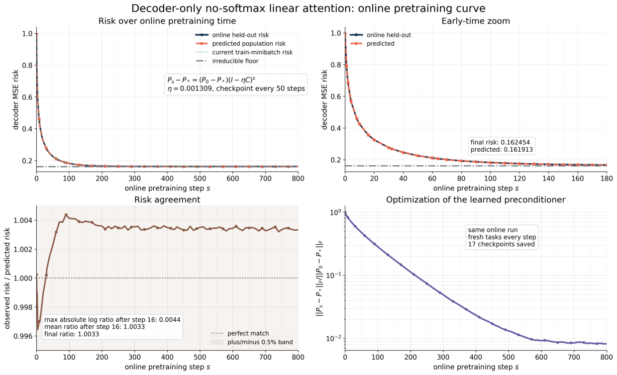 This curve is the outer training view of the same statement. The learned preconditioner improves during pretraining before it is frozen and reused as an inner solver. 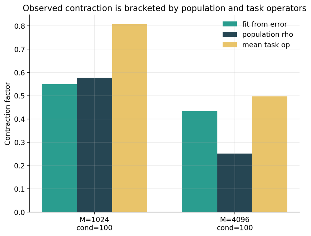 The contraction-factor diagnostic checks the exact Richardson certificate: smaller \(\|I-P_\theta A\|\) means fewer decoder layers are needed for the same right-hand-side accuracy.For fixed (P_\theta), the optimization certificate is exact:
\[\|e_L\|_2\le \|I-P_\theta A\|_2^L\|e_0\|_2.\]This explains why preconditioning matters. If (P_\theta=\eta I), convergence slows down when (A) is ill-conditioned. If (P_\theta\approx A^{-1}), the contraction (I-P_\theta A) becomes small and the same number of layers gives a much lower error.
In transformer language, attention is useful when it routes residual information into directions where the system is hard. The values carry residuals. The query-key scores decide which equations or spectral directions matter. The feed-forward block turns the routed residual information into a preconditioned correction.
For the constant-coefficient case, this is already enough: the whole problem collapses to learning a reusable solver for one Galerkin matrix.
What the prompt contributes
In this setting, the prompt does not need to identify a new coefficient field. It is better to think of it as calibration data for the solver behavior. Each pair ((f_i,u_i)) tells the model what the inverse map (f\mapsto u) looks like on another right-hand side. If the source distribution concentrates on a low-dimensional subspace, the prompt reveals which directions are common. If the source distribution is broad, the prompt pushes the model toward a more uniform approximation of (A^{-1}).
This is also the regime where the distinction between approximation and optimization is cleanest. The approximation question is whether the network class can represent a good (P_\theta). The optimization question is what happens after a particular (P_\theta) is fixed. The latter is completely answered by
\[e_L=(I-P_\theta A)^L e_0.\]There is no hidden transformer mystery in the frozen decoder. Once the model is interpreted as a recurrent solver, its depth-(L) error is exactly the error of (L) preconditioned Richardson steps.
Generalization in the constant case
The held-out risk is measured on fresh right-hand sides. With clipped loss (\ell_c=\min(\ell,c)), the finite-sample certificate is
\[R_c\leq \widehat R_c+ \sqrt{\frac{2\widehat V_c\log(2/\delta)}{n}} + \frac{7c\log(2/\delta)}{3(n-1)}.\]The clipping is not cosmetic. Raw squared Gaussian losses are unbounded, so a distribution-free statement needs either clipping or an explicit tail assumption. The experiments report both the raw risk and the clipped certificate.
In this constant-(A) regime, the expected scaling is simple. More decoder depth reduces the solver term like (\rho^{2L}). More pretraining tasks reduce uncertainty about the reusable preconditioner. More prompt examples help only to the extent that the architecture uses them to infer the active source subspace; they do not need to identify a new operator.
This is why the constant-coefficient case is the correct first sanity check. If the decoder cannot learn a useful preconditioner for one fixed Galerkin matrix, then the variable-coefficient task is premature. If it can, then the next question is how to encode the operator before applying the same solver logic.
What this says about attention
In the constant case, the most honest description of attention is not that it “solves the PDE” directly. Rather, it organizes residual information. If the tokens contain weak equations, a query can ask which equations are informative for a direction of the coefficient space. A value can carry the residual in that equation. The output projection and feed-forward block then turn the routed residuals into a correction.
For no-softmax linear attention, this story is especially literal: with enough head dimension, the attention block can reconstruct signed moments of the form
\[G^\top r.\]For softmax attention, positive normalization changes the algebra. Softmax is still useful as a routing mechanism, but the signed information must be carried carefully by the value stream or by paired positive/negative queries. This is why the experiments distinguish low-rank values, projected values, and full vector values.
The constant-coefficient setting is therefore a microscope. It isolates whether attention and the feed-forward block can implement a preconditioned residual update before any variable-coefficient inference is added. When the learned preconditioner decreases risk across held-out right-hand sides, it is evidence that the architecture has learned a solver primitive rather than a collection of task-specific answers.
Takeaway
The constant-(a) story is: one Galerkin matrix, many right-hand sides, one reusable learned preconditioner. The exact frozen optimization law is Richardson. The generalization test is held-out source prediction. This is the base case on which the variable-(a) encoder is built.
External Papers Used
This series uses paper names only after introducing the problem they solve. The main external anchors are the following.
Low-rank in-context learning and replica theory. Kaito Takanami, Takashi Takahashi, and Yoshiyuki Kabashima, “Learning Linear Regression with Low-Rank Tasks In-Context,” arXiv:2510.04548. This is the reference for the high-dimensional low-rank task model and its replica generalization calculation.
Training dynamics of linear attention. Yedi Zhang, Aaditya K. Singh, Peter E. Latham, and Andrew Saxe, “Training Dynamics of In-Context Learning in Linear Attention,” arXiv:2501.16265. This is the reference point for exact gradient-flow phenomena in linear-attention ICL.
Learnable linear-attention kernels. Haoran Zhang and Feng Zhou, “Flexformer: Flexible Linear Transformer with Learnable Attention Kernel,” arXiv:2606.27748. This motivates the learned-kernel decoder experiments, but the posts distinguish local diagnostics from a proved global training theory.
Differentiable Galerkin assembly. Shizheng Wen, Mingyuan Chi, Tianwei Yu, Ben Moseley, Mike Yan Michelis, Pu Ren, Hao Sun, and Siddhartha Mishra, “Learning, Solving and Optimizing PDEs with TensorGalerkin,” arXiv:2602.05052. This is the relevant numerical-analysis reference for differentiable Galerkin assembly and PDE-constrained learning.